Adding titles and axis labels

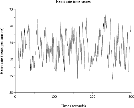
Now that we know how to make simple screen and printed plots, let's refine the plot a bit. First, we can provide a title for the plot, and for the x and y axes using the -t, -x, and -y options, like this:

plt heartrate.data -t "Heart rate time series" \
  -x "Time (seconds)" -y "Heart rate (beats per minute)"

(The ``$\backslash$'' at the end of the first line means that the command is continued on the next line; you may enter the command on two lines, ending the first with a backslash, or you may combine both lines into one, omitting the backslash.)

This command produces the neatly labelled version of the plot shown in figure 2.4. This and all of the later figures in this book were prepared as PostScript plots, using plt's ``-T lw'' option and piping the output to lwcat as in figure 2.3. Except in the discussion of printed output in appendix B, however, the plt commands shown here omit ``-T lw | lwcat'', so that they can be used to make screen plots.

Figure 2.4: Simple plot with titles and axis labels