Human cardiac dynamics are driven by the complex nonlinear interactions of two competing forces: sympathetic stimulation increases and parasympathetic stimulation decreases heart rate. For this type of intrinsically noisy system, it may be useful to simplify the dynamics via mapping the output to binary sequences, where the increase and decrease of the inter-beat intervals are denoted by 1 and 0, respectively. The resulting binary sequence retains important features of the dynamics generated by the underlying control system, but is tractable enough to be analyzed as a symbolic sequence.
Consider an inter-beat interval time series,
![]() , where
, where ![]() is the
is the ![]() -th inter-beat interval. We can classify each
pair of successive inter-beat intervals into one of the two states that
represents a decrease in
-th inter-beat interval. We can classify each
pair of successive inter-beat intervals into one of the two states that
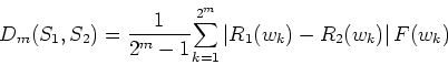
represents a decrease in ![]() , or an increase in
, or an increase in ![]() . These two states are
mapped to the symbols 0 and 1, respectively
. These two states are
mapped to the symbols 0 and 1, respectively
![\includegraphics[width=4in]{fig1a.ps}](img8.png) |
We map ![]() successive intervals to a binary sequence of length
successive intervals to a binary sequence of length ![]() ,
called an
,
called an ![]() -bit ``word.'' Each
-bit ``word.'' Each ![]() -bit word,
-bit word, ![]() , therefore, represents a
unique pattern of fluctuations in a given time series. By shifting one
data point at a time, the algorithm produces a collection of
, therefore, represents a
unique pattern of fluctuations in a given time series. By shifting one
data point at a time, the algorithm produces a collection of ![]() -bit
words over the whole time series. Therefore, it is plausible that the
occurrence of these
-bit
words over the whole time series. Therefore, it is plausible that the
occurrence of these ![]() -bit words reflects the underlying dynamics of
the original time series. Different types of dynamics thus produce
different distributions of these
-bit words reflects the underlying dynamics of
the original time series. Different types of dynamics thus produce
different distributions of these ![]() -bit words.
-bit words.
In studies of natural languages, it has been observed that authors have characteristic preferences for the words they use with higher frequency. To apply this concept to symbolic sequences mapped from the inter-beat interval time series, we count the occurrences of different words, and then sort them in descending order by frequency of occurrence.
The resulting rank-frequency distribution, therefore, represents the statistical hierarchy of symbolic words of the original time series. For example, the first rank word corresponds to one type of fluctuation which is the most frequent pattern in the time series. In contrast, the last rank word defines the most unlikely pattern in the time series.
To define a measurement of similarity between two signals, we plot the
rank number of each ![]() -bit word in the first time series against that
of the second time series.
-bit word in the first time series against that
of the second time series.
![\includegraphics[width=3in, clip]{fig2.ps}](img13.png) |
If two time series are similar in their rank order of the words, the
scattered points will be located near the diagonal line. Therefore,
the average deviation of these scattered points away from the diagonal
line is a measure of the ``distance'' between these two time
series. Greater distance indicates less similarity and vice versa. In
addition, we incorporate the likelihood of each word in the following
definition of a weighted distance, ![]() , between two symbolic
sequences,
, between two symbolic
sequences, ![]() and
and ![]() .
.
Here ![]() and
and ![]() represent probability and rank of a
specific word,
represent probability and rank of a
specific word, ![]() , in time series
, in time series ![]() . Similarly,
. Similarly, ![]() and
and
![]() stand for probability and rank of the same
stand for probability and rank of the same ![]() -bit word in
time series
-bit word in
time series ![]() . The absolute difference of ranks is multiplied by
the normalized probabilities as a weighted sum by using Shannon
entropy as the weighting factor. Finally, the sum is divided by the
value
. The absolute difference of ranks is multiplied by
the normalized probabilities as a weighted sum by using Shannon
entropy as the weighting factor. Finally, the sum is divided by the
value ![]() to keep the value in the same range of [0, 1]. The
normalization factor
to keep the value in the same range of [0, 1]. The
normalization factor ![]() in Eq. 3 is given by
in Eq. 3 is given by
![]() .
.
![\includegraphics[width=4in]{fig1c.ps}](img12.png)