Examples

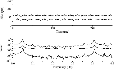
Several HR time series are presented below, together with the corresponding Lomb, FT, and AR spectra. In each case, an irregularly sampled instantaneous heart rate (IHR) signal was obtained from an RR interval time series using the algorithm given in the appendix, and this signal was used as input to the Press-Rybicki algorithm to obtain the Lomb periodogram. A regularly sampled instantaneous heart rate signal[3] was obtained from the same RR series; this signal (five minutes in length in each case, and sampled at 2 Hz) was zero-meaned, detrended, zero-padded to a length of 1024 samples, and Welch windowed, and the result was used as input to standard fast Fourier transform (FT) and autoregressive model (AR) algorithms for PSD estimation[11]. In the examples shown here, the AR models are of order 24. The Lomb and AR spectra can be evaluated for any desired frequencies; for purposes of comparison, all spectra were evaluated at the discrete frequencies defined for the Fourier spectra.

To demonstrate the essential similarity of FT, AR, and Lomb PSD estimates, synthesized HR time series are shown in Figures 1 and 2.

Figure 1: Synthesized HR time series and corresponding spectra (see text). In Figures 1-5, the upper trace is the resampled HR series used to derive the FT and AR spectra; below it is the IHR series (offset by 25 bpm for clarity) used to derive the Lomb spectrum. The lower panel shows, from top to bottom: the Lomb spectrum (heavy line); the AR spectrum (dotted line); and the FT spectrum (thin line). For clarity, the AR and FT spectra are offset by $10^{3}$ and $10^{6}$ units respectively.

These five-minute sequences were generated using a recurrence of the form

$$RR_{i} = a_{0} + a_{1} \sin ( {\omega_{1} t_{i} + \phi_{1}} ) + a_{2} \sin ( {\omega_{2} t_{i} + \phi_{2}} ) + a_{3} z$$ (1)

$$t_{i+1} = t_{i} + RR_{i}$$ (2)

where $RR_{i}$ is the RR interval beginning at $t_{i}$, $z$ is a random variable evenly distributed between -1 and 1, and the remaining parameters are arbitrary constants. For the simulation shown in Figure 1, both $a_{1}$ and $a_{2}$ are 0, so that the sequence contains randomly-varying intervals with a mean of $a_0$ (1 second in the simulations shown here). The Lomb periodogram of this sequence is consistent with white noise, whereas the FT and AR spectra show the high-frequency (HF) attenuation expected as a result of the resampling process. In Figure 2, $a_{1}$ and $a_{2}$ are equal and larger than $a_{3}$; $\omega_{1}$ and $\omega_{2}$ are chosen to modulate the RR intervals at frequencies of 0.05 and 0.41 Hz, to simulate sympathetically-mediated low frequency HR oscillations and parasympathetically-mediated respiratory sinus arrhythmia. The three spectra are quite similar, apart from the HF attenuation in the FT and AR spectra, and the lack of detail/clutter in the AR spectrum.

Figure 2: Synthesized HR time series and corresponding spectra (see text).

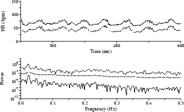
The sequence in Figure 3 was obtained by automated analysis of an ECG signal acquired from a subject with sleep apnea syndrome; the low frequency modulation of heart rate with a period of roughly 45 seconds matches the frequency of the subject's obstructive apneas. Although the spectral peak near 0.025 Hz is most obvious in the AR spectrum, it is also clearly visible in both the Lomb and the FT spectra, which also reveal the harmonically related peak near 0.05 Hz.

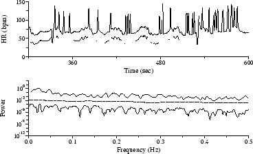
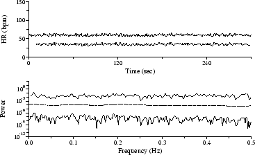
The sequence in Figure 4 was obtained by automated analysis of the same signal used in Figure 3, after addition of electrode motion artifact scaled to obtain a signal-to-noise ratio of 12 dB. Roughly 30 QRS detector errors resulting from the added noise are readily discernible in the time series. Although much of the sequence is rejected by the algorithm that prepares input for the Lomb periodogram, the peak near 0.025 Hz is still prominent, and the first harmonic also remains visible. The 0.025 Hz peak is visible but not significant among the clutter in the FT spectrum, and the AR spectrum has no significant features.

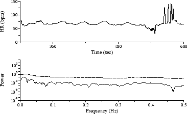
By rejecting the outliers and using a predictive interpolator to obtain replacement samples, as shown in Figure 5, the 0.025 Hz peak emerges as a broad feature in the AR spectrum, but the FT spectrum shows a broad, spurious peak at about 0.015 Hz.

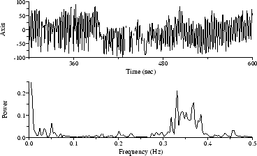
Other irregularly-sampled time series frequently appear in HRV-related studies. Among those amenable to Lomb PSD analysis are respiration intervals and tidal volumes, gait, and beat-by-beat systolic blood pressure measurements. As a final example, Figure 6 shows a time series of beat-by-beat measurements of the mean cardiac electrical axis, which fluctuates in response to respiration[12]; the Lomb spectrum clearly reveals the respiratory frequency.

Figure 3: HR time series and spectra during periodic obstructive apneas.

Figure 4: HR time series from Figure 3, corrupted by added noise, with corresponding spectra.

Figure 5: HR time series from Figure 4, corrected using a predictive interpolator, with corresponding AR and FT spectra.

Figure 6: Electrical axis time series (above), with Lomb spectrum (below).