Plotting Data

Most of the previous examples have illustrated how two columns of data can be plotted as a connected set of line segments. This is plt's default style for plotting data, but many other styles are supported using the -p option to choose a plotstyle. For example, data can be plotted using points, characters, strings, or symbols (scatter plots); with error bars; or using lines of various widths, grey levels, colors, or patterns (solid, dotted, etc.).

To specify a plotstyle, we can use the -p option, followed by sub-options that control how the points are plotted. Each sub-option can also have an optional argument following it. This argument can change the font, point size, color, gray scale, line width, or line style (solid, dotted, dashed, etc.) of the current plot. (If you want to use those control options that enable you to make font changes, you will need to read and understand chapter 11, Colors, Line Styles, and Fonts, beginning on page .)

Each plotstyle ``takes'' (consumes) one or more data columns. If you use more than one plotstyle, you must include enough data column numbers for all of the plotstyles in the plt command line. Note that you may repeat data column numbers if necessary to satisfy the requirements of the plotstyles you select; see the examples below to see how this can be done.

If you have not used plt previously, it is probably a bad idea to read through this chapter from beginning to end, because the usage of the plotstyles (especially the first one listed below, c) is mind-bogglingly convoluted. A better strategy is to begin by studying the examples in this chapter; find one or more that illustrate features you would like to use in your own plots, then see which plotstyles were used to obtain these features.

The sub-options to -p are:

c

Takes three data columns ($x$, $y$, and $c$). Each $c$ value tells plt what to do with the corresponding $x$ and $y$ values. The values for $c$ can be:

0	continue (draw) path to $(x,y)$
1	move to $(x,y)$ without drawing (i.e., with the ``pen'' up), then put the pen down (begin a new path)
2	put a dot at $(x,y)$
3	put a small box at $(x,y)$
9	paint the path (usually done as the default when a new path is begun without specifying what to do with the old one)
10	continue to $(x,y)$, close path and fill the inside with grey level specified by the argument to the c sub-option
11	continue to $(x,y)$, close path and fill the inside with grey level specified by the argument to the c sub-option; then draw a black border
12 - 13	continue to $(x,y)$, close path and fill the inside with grey level specified by $c-12$ (12.0 = black, 13.0 = white)
14 - 15	continue to $(x,y)$, close path and fill the inside with grey level specified by $c-14$ (14.0 = black, 15.0 = white); then draw a black border
20	(requires -fs option, see section 3.7, String arrays, page ) change font to that specified by string number $x$ from the -fs string array
21	change point size to $x$
22	change line width to $x$
23	(requires -fs option, see section 3.7) change line style to that specified by string number $x$ from the -fs string array; legal line styles are ``solid'', ``dotted'', ``shortdashed'', ``dotdashed'', and ``longdashed''. Note that $y$ is ignored (see figure 6.1).
24	change grey level to $x$ (0 = black, 1 = white); $y$ is ignored.
25	(requires -fs option, see section 3.7) change color to that specified by string number $x$ from the fontgroup string array (see appendix A for details on how to specify colors by name; also, note that $y$ is ignored)
30 - 39	put symbol number $c-30$ at $(x,y)$ (see figure 6.2)
100, 101, ...	(requires -tf or -ts option, see section 3.7) put string number control-100 from the text string array at $(x,y)$

Figure 6.1: Produced using the command:

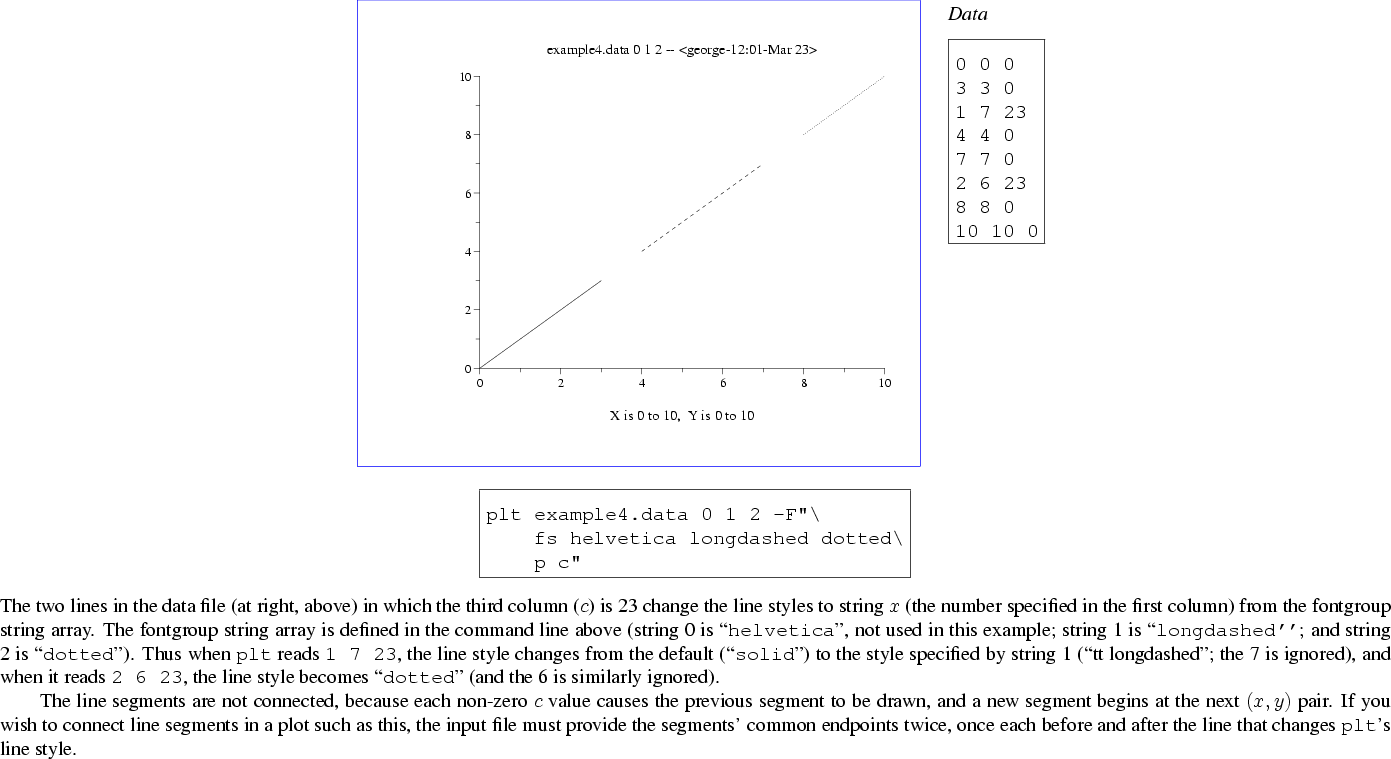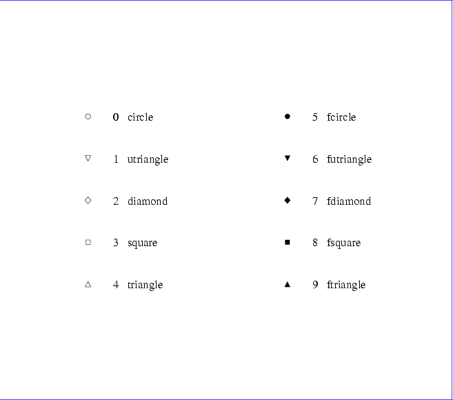
Figure 6.2: The ten symbolsthat can be plotted using plotstyles c (suboptions 30 through 39), E, and S. Numeric (0-9) and mnemonic (``circle'', ``square'', etc.) names appear to the right of each symbol; either form may be used when specifying a symbol to be used with plotstyles E or S. The open symbols (0 through 4) have opaque centers; these are particularly recommended for relatively dense scatter plots because it is still possible to distinguish and count individual data points even when the symbols partially overlap. The size of the symbols is determined by the current font's point size (see the description of the -sf option in chapter 11), Colors, Line Styles, and Fonts, beginning on page .

C

Takes two columns, $x$ and $y$, assumed to be the vertices of a polygon. The polygon is drawn by connecting consecutive vertices and by connecting the last vertex to the first, and then it is filled in the current color (default: black). Nonconvex and self-intersecting polygons are filled properly. See figure 6.3, page .

e+$c$

Takes three columns ($x$, $y$, and $e$). This sub-option makes a scatter plot, like s (see below), but including error bars. Each $e$ value tells plt the size of the error associated with the corresponding $x$ and $y$. When using the e sub-option, you may specify the character (default: ``*'') to use when plotting $(x,y)$, and you must indicate if you wish to plot the top, bottom, or both halves of the error bars, as follows:

e-$c$

e:$c$

 

e+$c$

plot $(x,y)$ as ``$c$'', with top half of error bars only

e-$c$

plot $(x,y)$ as ``$c$'', with bottom half of error bars only

e:$c$

plot $(x,y)$ as ``$c$'', with both top and bottom error bars; the ``:'' may be omitted unless $c$ is either ``+'' or ``-''

E+$n$

Takes three columns ($x$, $y$, and $e$). Exactly like its counterpart, e, except that this sub-option allows you to plot a specified symbol (identified by a symbol number $n$ between 0 and 9 inclusive) instead of a character.

E-$n$

E:$n$

 

f

Takes three columns ($x$, $y_0$, and $y_1$) and fills the area defined by the normal plots of $(x,y_0)$ and $(x,y_1)$ in the current color (default: black). See figure 6.10, page .

i

Takes two columns, $x$ and $y$. The $(x,y)$ pairs are plotted in impulse response form. See figure 6.11, page .

l

Takes four columns, $x_{0}$, $y_{0}$, $x_{1}$, and $y_{1}$. The line segments with endpoints $(x_{0},y_{0})$ and $(x_{1},y_{1})$ are plotted. See figure 6.12, page .

m

Takes one column ($y$). The $x$ values are always taken from column 0 of the input. The output is a normal plot of $(x,y)$ pairs. (If you supply only one data column number to plt and do not specify a plotstyle, this is the type of plot you will obtain by default.) See figure 6.13, page .

n

Takes two columns, $x$ and $y$. The output is a normal plot of $(x,y)$ pairs. (If you supply two data column numbers to plt and do not specify a plotstyle, this is the type of plot you will obtain by default.) See figure 6.14, page .

N

Takes two columns, $x$ and $y$. The area bounded by the normal plot of the $(x,y)$ pairs and the x axis is filled with the current color (default: black). See figure 6.15, page .

o

Takes three columns ($x$, $y_0$, and $y_1$) and outlines the area defined by the normal plots of $(x,y_0)$ and $(x,y_1)$ in the current color (default: black). See figure 6.16, page .

O

Takes three columns ($x$, $y_0$, and $y_1$), outlines the area defined by the normal plots of $(x,y_0)$ and $(x,y_1)$ in black, and fills this area in the current color (default: black). See figure 6.17, page .

s$c$

Takes two columns, $x$ and $y$. The output is a scatter plot of $(x,y)$ pairs, where each pair is plotted using the character specified by $c$ (a character suffixed to the plotstyle name, s). See figure 6.18, page .

S$n$

Takes two columns, $x$ and $y$. Exactly like its counterpart, s, except that this plotstyle allows you to plot a specified symbol (identified by a symbol number $n$ between 0 and 9 inclusive), instead of a character. See figure 6.19, page .

t

Takes three columns, $x$, $y$, and $n$. This plotstyle must be used together with the -tf or -ts option (see section 3.7). The $n$ values specify strings from the -tf or -ts string array; plt prints these at the locations given by the corresponding $(x,y)$ pairs (adjusting the string positions according to the text box coordinates provided to the -tf or -ts option). See figure 6.20, page .