Interacting with Scilab

In the previous chapter we were able to edit an annotation file, modifying the QRS complexes detected by WFDB software. Now we want to export the results to be used with other software.

As you probably know, Scilab is a Matlab-like scientific software package for numerical computation that can be very useful in managing neurophysiological signals. In this section we are going to try to link signals and annotations between WFDB tools and Scilab.

In the last chapters we were able to convert ASCII files containing matrices of data into WFDB files. Matrices are the core of Scilab. Managing matrices (even very long ones) is extremely easy in Scilab. Since a recording can be seen as a matrix of values (the columns being signals), ASCII files, once more, can be used as the glue to connect Scilab and WFDB.

Reading the results of processing with Scilab

Our first task is to create a signal containing the heart rate. We would like for this signal to be sampled at the same rate as the ECG signal. WFDB has an application named tach that can make a heart rate tachogram from an annotation file. We can use tach to make either a WFDB-format tachogram that can be studied with wave, or a text-format tachogram that we can study with Scilab. We are going to indicate that we want the heart rate signal sampled at 200 Hz (the sampling rate of the original signal), and we send the result to the file tac.

[j@localhost Code]$ tach -r ecg -a qrs -F 200 > tac

Let us see how easy is to read the result with Scilab. We call Scilab from the same directory. Now we will read the file base containing the original signals and the file tac that contains the result of our analysis

[j@localhost Code]$ scilab 
                           ===========
                           S c i l a b
                           ===========


                          scilab-2.6
                  Copyright (C) 1989-2001 INRIA


Startup execution:
  loading initial environment

-->tac = fscanfMat("tac");

-->size(tac)
 ans  =

!   3241.    1. !

-->base = fscanfMat("base");

-->size(base)
 ans  =

!   3400.    19. !

Now we have two variables in Scilab:

• base: This is a matrix with 19 signals (columns). In the column 10 (9 for WFDB since WFDB counts from 0) we have the ECG that was analyzed.
• tac: This is a column of values containing the tachogram.

We can plot it:

-->time1 = (1:3241)/200;

-->signal1 = tac;

-->time2 = (1:3400)/200;

-->signal2 = base(:,10);

-->plot2d(time1,signal1)

-->plot2d(time2,signal2/5)

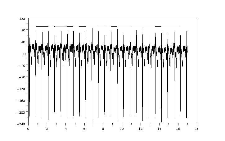
The result can be seen in figure 4.1.

Figure 4.1: The tachogram plotted together with the ECG in Scilab

We have corrected the amplitude of the electrocardiographic signal. There is a good coincidence between the ECG and the heart rate. You can check the result by eliminating in wave some QRS detections and by observing the changes with Scilab.

WFDB is very well equipped to analyze electrocardiographic signals. We are going to make some analysis not implemented in WFDB. We want to detect the respiratory rate. We have the airway signal in column 14 (13 in WFDB) of our original recording (base).

Creating some analysis tools with Scilab

To analyze the respiratory rate with Scilab we will use a very simple approach. Do not pay to much attention to the details since we are using it only as an example of an alternative analysis made with Scilab.

The approach includes the following steps:

• We read the file base into Scilab's variable base
• We extract the column containing the respiratory signal to the Scilab's variable res
• We detect the points that exceed an amplitude of 60 (our signal fluctuates from -140 to 140). Now we have a vector (over60) that contains the value 1 at the points that are over 60 and a value 0 in each other point
• We detect the transitions from 0 to 1 by subtracting from each point the previous one.
• We store the transitions as an index vector (called ndx). This index stores the point where a trigger detecting the level of 60 in increasing direction would be placed.

Let us see the code (note that Scilab code is less verbose than the explanation):

  
-->base = fscanfMat("base");             // reading the file
 
-->res = base(:,14);                     // extracting column 14
 
-->over60 = 1*(res>60);                  // values over 60
 
-->changes = over60(2:$)-over60(1:$-1);  // changes can be -1, 0 ,1 
 
-->ndx = find( changes >0 )              // detection of values 1
 ndx  =
 
!   342.    884.    1435.    1936.    2445.    2957.

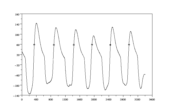
Let us check the result by plotting the detection with the respiratory signal

-->plot(res)                              // the respiratory signal
 
-->plot2d(ndx,res(ndx),-3)                // plotting ndx as points

The result can be seen in figure 4.2.

Figure 4.2: The respiration signal marked with the detection

As we can see, the marked points act as a trigger. But if we want to see the result in wave, it is not an easy task: we have to create a WFDB annotation file.

Trying to create an annotation file with the result

To create an annotation file, our first thought is using wrann. Given our success by using wrsamp we could try this approach.

Let's see the information about wrann:

The usual application for wrann is as an aid to annotation file 
editing: an annotation file may be translated into ASCII format
using rdann, edited using a text editor, and then translated back
into annotation file format using wrann.

So wrann has been conceived to allow editing with a text editor. It seems a dead end. We would like to have a tool to create annotations easily from Scilab. We could follow the following approaches:

• We can understand the annotation format (it is completely documented) and program an application from scratch, even using Scilab. It would not be very convenient. It is a difficult task and we try to use as much previous code as possible.
• We could program an application by using the WFDB library. It is a very professional approach. It is difficult but the result is the best. We could even send our code to PhysioNet and, eventually, it could be considered for wider diffusion
• We could modify wrann to be adapted to our needs. It is much simpler. If we need to create a lot of annotations, probably it is the best choice but we will have a non-standard application
• We could create some output that mimics the output of rdann by using an editor. It is the simplest approach.
• We could try to understand the machinery of wrann to create some file that can be understood by wrann

Having a lot of possibilities increases the probability of error (Do you remember the simple camera of the introduction?). WFDB is open source software. Let us explore the code of wrann. After some searching, we reach to the core of the interface with the external files (lines 111 to 113):

    while (fgets(line, sizeof(line), stdin) != NULL) {
	p = line+9;
	if (line[0] == '[')
	    while (*p != ']')
		p++;
	while (*p != ' ')
	    p++;
	(void)sscanf(p+1, "%ld%s%d%d%d", &tm, annstr, &sub, &ch, &nm);
	annot.anntyp = strann(annstr);
	annot.time = tm; annot.subtyp = sub; annot.chan = ch; annot.num = nm;
   ...

So, it seems that a line is read and unless the first character of the line is an square bracket it skips the first 9 characters and uses the C function sscanf to read a long integer (the position of the annotation), a string (the type) and three integers (the subtype, the chan and the num field). Probably, knowing the sample, the remainder of the annotation can be reconstructed. We could try to write some code to emulate the input format of wrann from Scilab.To do this, we create a string with the format. Let us see the code (the first lines have been repeated for convenience):

  
-->base = fscanfMat("base");
 
-->res = base(:,14);
 
-->over60 = 1*(res>60);
 
-->changes = over60(2:$)-over60(1:$-1);
 
-->ndx = find( changes >0 )
 ndx  =
 
!   342.    884.    1435.    1936.    2445.    2957. !
 
-->format_ann = "**dummy** %13.0f [15] 0 0 0";   // our discovery
 
-->fprintfMat("dummy_file",ndx',format_ann);     // store to a file

Notice that **dummy** has exactly 9 characters. We choose [15] because it is an unassigned annotation type. Our creature begins to live. Now we have to check the result (we return to the terminal):

 
[j@localhost Code]$ cat dummy_file
**dummy**           342 [15] 0 0 0
**dummy**           884 [15] 0 0 0
**dummy**          1435 [15] 0 0 0
**dummy**          1936 [15] 0 0 0
**dummy**          2445 [15] 0 0 0
**dummy**          2957 [15] 0 0 0
[j@localhost Code]$ cat dummy_file | wrann -r ecg -a res
[j@localhost Code]$ rdann -r ecg -a res
    0:01.710      342  [15]    0    0    0
    0:04.420      884  [15]    0    0    0
    0:07.175     1435  [15]    0    0    0
    0:09.680     1936  [15]    0    0    0
    0:12.225     2445  [15]    0    0    0
    0:14.785     2957  [15]    0    0    0

Isn't it incredible? We introduce garbage and we receive annotations properly formatted. Let's check that our method functions:

 
[j@localhost Code]$ wave -r ecg -a res

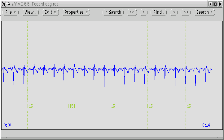
We select the record ecg.dat with the annotation file ecg.res.

The result can be seen in figure 4.3.

Figure 4.3: In this ocasion the ECG is plotted together with the marks of the respiratory cycle

After some arrangements, we were able to introduce the result of the analysis. We have the ECG with the position of the respiratory cycle marked in the same screen. If we had plotted the respiratory signal (a trivial task), we could begin a new cycle of editing and exporting results. Our analysis was trivial (a trigger to detect the respiration cycle), but by using the same approach you can mark anything in the file of your commercial equipment (if it exports ASCII files) and edit the result in wave. Let us mention some things that you can mark:

• arousals
• K-complexes
• spindles
• apneas
• external stimuli...

And many more. Would you not like to see whether the temporal pattern of spindles is modified by drugs? What is the temporal relation between K-complexes and spindles? Do really spindles decrease in slow wave sleep or are they masked by the EEG? Does the auditory evoked potential relate with the sleep stages? These are questions that you can explore with WFDB software.

Using Scilab as a tool from wave

Wave uses a very ingenious method for further processing. Let us adapt it to use Scilab. We define the editor (any other editor can be used) and call wave:

[j@localhost Code]$ export EDITOR=/usr/openwin/bin/textedit
[j@localhost Code]$ wave -r 100s

Then you click on File > Analyze and a Notice appears indicating that the file wavemenu will be copied in your directory. Once you choose Copy, you can begin to edit the menu. At the end you add the following lines:

...
# list contains three signals).  Adjust the -rx and -rz options to obtain the
# desired viewpoint.

# Add additional entries below.
Hello Scilab   	echo "key= x_message (\"You are reading record $RECORD\" ) " \
                > com.sce; \
		echo "exit()" >> com.sce; \
		scilab -nw -f com.sce

The main features of the connection are illustrated here:

• Scilab is called with the option -nw, so it does not initiate a new window.
• Scilab is called with the option -f, so it reads the file indicated (com.sce).
• We create the file by echoing strings from Wave; notice that the variables from Wave can be passed to Scilab.
• We could indicate to Scilab that any other file (with complex processing commands) must be loaded and executed.

Now you save the file and click Reread menu in the Analyze window. A new button called Hello Scilab appears. If you click it, a small window with a message indicating the file that you are processing appears.

Do not pay too much atention to this subsection. A lot of things can fail with this approach: Scilab must be installed, you have to be in the proper directory, you have to be able to write the file (com.sce) and above all the synthax is very difficult. It is much better to call scilab from the command line. This point was included only to show the versatility of Wave.

In summary

In this section we were able to mix the analysis made by external programs with some elementary analysis made by Scilab. Scilab is a general mathematical package, Wave is a friendly viewer with a lot of powerful possibilities, WFDB applications are a set of very well conceived and checked programs for signal and annotation processing and analysis, including many designed for electrocardiographic analysis. In this chapter we made them work together by acting on ASCII files.