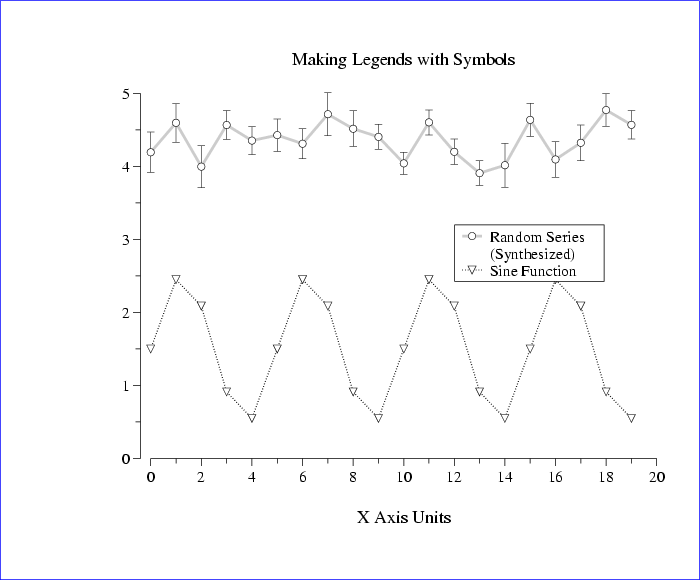
A legend (also known as a key) is useful when two or more data plots are drawn on the same axes, as in the previous section. A legend typically includes sample plot segments (short segments drawn using the same line styles used for the data plots), each of which is followed by legend text (typically a description of the associated plot). Figure 7.3 illustrates a plot that includes a boxed legend.
The -lp option is used to specify the location for the legend, and the -le option is used to define an entry to be shown as part of the legend. These options take their arguments as follows:
-lp xw0 yw0 boxscale seglength opaque
-le linenumber plotnumber text
The first two arguments of -lp define the window coordinates of the upper left corner (LT) of the legend text. plt draws a box around the legend text, determining the width and height of the box based on the size of the text and sample plot segments it encloses, but you can adjust the width of the box using the optional boxscale argument (which is a factor that multiplies the width calculated by plt). Thus a boxscale of 1.05 creates a box 5% larger than the default size; as a special case, a boxscale of 0 suppresses the box entirely. The optional seglength argument tells plt how long to make the sample plot segments in the legend, as a fraction of the x axis length (by default, plt draws these segments so that they are 5% of the length of the x axis). If opaque is yes (default), the background of the legend box is opaque white; otherwise, the legend box is transparent (any previously drawn material remains visible through the legend box).
The first argument of -le specifies the line number of the entry within the legend (the top line is line number 0). Each plot drawn by plt has an implicit plotnumber (the first has a plotnumber of 0); this is the second argument of -le, used to determine the line style for the entry's sample plot segment). The third and final argument of -le is the text to be shown next to the sample plot segment.
Study figure 7.3 to see how these options work. This plot was produced using the command
plt example10.data % -f example10.formatwhere the data file, example10.data, was produced by this program fragment:
for (i = 0; i < 20; i++)
    printf("%d %.3lf %.3lf %.3lf\n",
           i,
           sin(0.4*i*PI) + 1.5,
           (double)random()/(double)RAND_MAX + 3.8,
           .1 + 0.15*(double)random()/(double)RAND_MAX);
and example10.format contains:
t Making Legends with Symbols
x X Axis Units
xa 0 20 1
ya 0 5

# Move the y axis slightly to the left.
yo .02

# Make four plots on the same set of axes.
p 0,1n(W5,L1) 0,1S1 0,2n(W12,G.8) 0,2,3E0

# Put legend text at window coordinates (.67,.64) and
# widen the legend box by 5%.
lp .67 .64 1.05

# Describe plot 2 in the top line (line 0) of the legend.
le 0 2 Random Series

# Plot 3 is the same as plot 2, but with a different
# plotstyle (using symbols).  By using a second "le"
# command for line 0 here, we create a sample plot
# segment that is composed by overlaying the two
# plotstyles.  The text has already been supplied in
# the previous command, so it is omitted here.
le 0 3

# The plot number is omitted from the next "le" command,
# because the text that is to appear on line 1 of the
# legend is a continuation of the description of the
# data in line 0.  The "-" means that no sample data
# segment will be drawn when this command is executed.
le 1 - (Synthesized)

# Describe plots 0 and 1.
le 2 0 Sine Function
le 2 1
(The -yo option is described in chapter 12.) The line beginning with ``p 0...'' makes four plots using several different plot styles:
Transient fontgroup modifications such as ``(W5,L1)'' and ``(W12,G.8)'' are described in detail in chapter 11. Note that the order of the overlay affects the appearance; since the open symbols (numbers 0 through 4) used in plots 1 and 3 have opaque centers, they appear differently if drawn on top of (after) other elements than if drawn below (before) those elements.