


Next: Conclusions
Up: Signals with different local
Previous: Dependence on the size
Scaling Expressions
To better understand the complexity in the scaling behavior of components
with correlated and anti-correlated segments at different scales, we employ
the superposition rule (see [61] and Appendix 7.1). For each
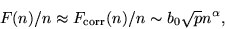
component we have
![\begin{displaymath}
F(n)/n=\sqrt{[F_{\rm corr}(n)/n]^2+[F_{\rm rand}(n)/n]^2},
\end{displaymath}](img131.png) |
(7) |
where
 accounts for the contribution of the correlated or
anti-correlated non-zero segments, and
accounts for the contribution of the correlated or
anti-correlated non-zero segments, and
 accounts for the
randomness due to ``jumps'' at the borders between non-zero and zero segments
in the component.
accounts for the
randomness due to ``jumps'' at the borders between non-zero and zero segments
in the component.
Components with correlated segments ( )
)
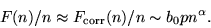
At small scales  , our findings presented in Fig. 6(b)
suggest that there is no substantial contribution from
. Thus
from Eq. (7),
, our findings presented in Fig. 6(b)
suggest that there is no substantial contribution from
. Thus
from Eq. (7),
 |
(8) |
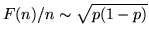
where  is the r.m.s. fluctuation function for stationary
(
is the r.m.s. fluctuation function for stationary
( ) correlated signals [Eq. (6) and [61]].
Similarly, at large scales  , we find that the contribution of
is negligible [see Fig. 7(a)], thus from
Eq. (7) we have
, we find that the contribution of
is negligible [see Fig. 7(a)], thus from
Eq. (7) we have
 |
(9) |
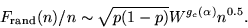
However, in the intermediate scale regime, the contribution of
to  is substantial. To confirm this we use the
superposition rule
[Eq. (7)] and our estimates for
at small
[Eq. (8)] and large [Eq. (9)] scales[65]. The result we
obtain from
is substantial. To confirm this we use the
superposition rule
[Eq. (7)] and our estimates for
at small
[Eq. (8)] and large [Eq. (9)] scales[65]. The result we
obtain from
![\begin{displaymath}
F_{\rm rand}(n)/n=\sqrt{[F(n)/n]^2-[b_0\sqrt{p}n^{\alpha}]^2-[b_0pn^{\alpha}]^2}
\end{displaymath}](img135.png) |
(10) |
overlaps with in the intermediate scale regime, exhibiting a
slope of  :
:
 [Fig. 9(a)]. Thus,
is indeed a contribution due to
the random jumps between the non-zero correlated segments and the zero
segments in the component [see Fig. 5(c)].
[Fig. 9(a)]. Thus,
is indeed a contribution due to
the random jumps between the non-zero correlated segments and the zero
segments in the component [see Fig. 5(c)].
Figure 9:
(a) Scaling behavior of components containing correlated segments
(). exhibits two crossovers and three scaling regimes
at small, intermediate and large scales. From the superposition rule
[Eq. (7)] we find that the small and large scale regimes are
controlled by the correlations ( ) in the segments
[
) in the segments
[
 from Eqs. (8) and (9)] while the
intermediate regime [
from Eqs. (8) and (9)] while the
intermediate regime [
 from Eq. (10)]
is dominated by the random jumps at the borders between non-zero and zero
segments. (b) The ratio
from Eq. (10)]
is dominated by the random jumps at the borders between non-zero and zero
segments. (b) The ratio
 in the
intermediate scale regime for fixed
in the
intermediate scale regime for fixed  and different values of
  , and
the ratio
, and
the ratio
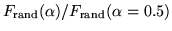 for fixed
and
for fixed
and  .
.
 is obtained from Eq. (10)
and the ratios are estimated for all scales
is obtained from Eq. (10)
and the ratios are estimated for all scales  in the intermediate regime.
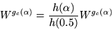
The two curves overlap for a broad range of values for the exponent ,
suggesting that
does not depend on
in the intermediate regime.
The two curves overlap for a broad range of values for the exponent ,
suggesting that
does not depend on  [see
Eqs. (11) and (16)].
[see
Eqs. (11) and (16)].
 |
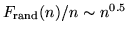
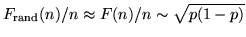
Further, our results in Fig. 8(b) suggest that in the intermediate
scale regime
 for fixed fraction [see
Sec. 5.2.2], where the
power-law exponent
for fixed fraction [see
Sec. 5.2.2], where the
power-law exponent  may be a
function of the scaling exponent characterizing the correlations in
the non-zero segments. Since at intermediate scales
dominates
the scaling [Eq. (10) and Fig. 9(a)], from
Eq. (7) we find
may be a
function of the scaling exponent characterizing the correlations in
the non-zero segments. Since at intermediate scales
dominates
the scaling [Eq. (10) and Fig. 9(a)], from
Eq. (7) we find
 . We also find that at intermediate scales,
 for fixed segment size
  (see Appendix 7.2,
Fig. 10). Thus from Eq. (7) we find
(see Appendix 7.2,
Fig. 10). Thus from Eq. (7) we find
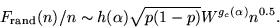
 . Hence we obtain the following general expression
 |
(11) |
Here we assume that
also depends directly on the type of
correlations in the segments through some function .
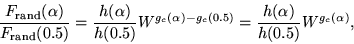
To determine the form of in Eq. (11), we perform the
following steps:
(a) We fix the values of and , and from Eq. (10) we
calculate the value of
for two different values of the
segment size , e.g., we choose  and
and  .
.
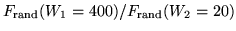
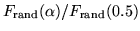
(b) From the expression in Eq. (11), at the same scale in the
intermediate scale regime we determine the ratio:
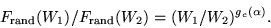 |
(12) |
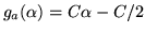
(c) We plot
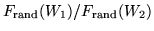 vs. on a linear-log scale
[Fig. 9(b)]. From the graph and Eq. (12) we obtain the
dependence
vs. on a linear-log scale
[Fig. 9(b)]. From the graph and Eq. (12) we obtain the
dependence
![\begin{displaymath}
g_c(\alpha)=\frac{\log[F_{\rm rand}(W_1)/F_{\rm rand}(W_2)]}...
... \leq 1$}\\
0.50, \mbox{ for $\alpha>1$},
\end{array} \right.
\end{displaymath}](img153.png) |
(13) |
where 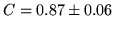 . Note that
  .
.
To determine if
depends on in Eq. (11), we
perform the following steps:
(a) We fix the values of and and
calculate the value of
for two different values of the
scaling exponent , e.g.,  and any other value of from
Eq. (10).
and any other value of from
Eq. (10).
(b) From the expression in Eq. (11), at the same scale in
the intermediate scale regime we determine the ratio:
 |
(14) |
since from Eq. (13).
(c) We plot
 vs. on a linear-log
scale [Fig. 9(b)] and find that when
vs. on a linear-log
scale [Fig. 9(b)] and find that when
 [in
Eqs. (12) and (14)] this curve
overlaps with
vs.
[Fig. 9(b)] for all values of the scaling exponent
[in
Eqs. (12) and (14)] this curve
overlaps with
vs.
[Fig. 9(b)] for all values of the scaling exponent
 . From this overlap and from Eqs. (12)
and (14), we obtain
. From this overlap and from Eqs. (12)
and (14), we obtain
 |
(15) |
for every value of , suggesting that
 and thus
can finally be expressed as:
and thus
can finally be expressed as:
 |
(16) |
Components with anti-correlated segments ( )
)
Our results in Fig. 6(a) suggest that at small
scales there is no substantial contribution of
and
that:
|
(17) |
a behavior similar to the one we find for components with correlated segments
[Eq. (8)].
In the intermediate and large scale regimes ( ), from the plots in
Fig. 7(b) and Fig. 8(a) we find the scaling behavior of
is controlled by
and thus
), from the plots in
Fig. 7(b) and Fig. 8(a) we find the scaling behavior of
is controlled by
and thus
 |
(18) |
where
 for
for  [see Fig. 9(b)] and
the relation for
is obtained using the same procedure we
followed for Eq. (16).
[see Fig. 9(b)] and
the relation for
is obtained using the same procedure we
followed for Eq. (16).
Next: Conclusions
Up: Signals with different local
Previous: Dependence on the size
Zhi Chen
2002-08-28