Viewing Examples

The following examples illustrate how to view waveforms and cardiac function/venous return curves on-line and off-line. Prior to implementing these examples, the researcher should set the time duration displayed by the WAVE window to 20 seconds by resizing the window and/or adjusting the Time scale variable (click VIEW option at the top of the WAVE menu bar).

Ex. 1

• Desired Execution:
  • On-line display of left ventricle pressure, volume, and flow rate.
  • Uncontrolled, unperturbed, intact pulsatile heart and circulation with default parameter values.
• Required Steps:
  1. Copy file $DIR/bin/parameters.def to the current directory with the new file name parameters_1.
  2. Open the file parameters_1 with any text editor (e.g., emacs).
  3. Re-assign the following parameters: waveform: 0 9 17 and annotations: 0. Make sure all of the status parameters are set to zero.
  4. Save the file parameters_1.
  5. Run the following command at the Linux prompt:
     rcvsim parameters_1 foo1
• Execution Output:
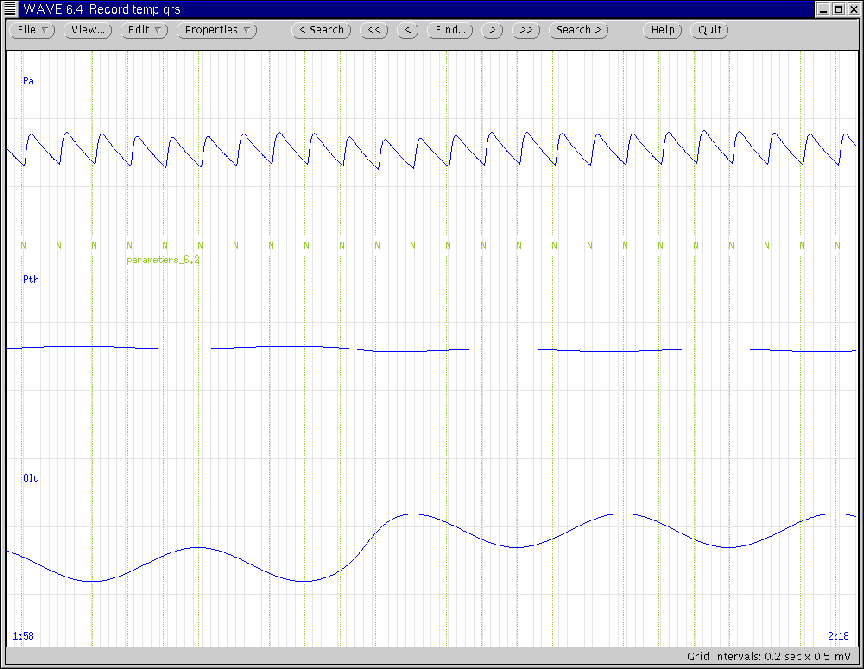
  • The WAVE window in Figure 10 will initially appear and will automatically scroll through the simulated data as they are being generated. This process will terminate once 300 seconds of the data have been simulated.
  • The following files will be created in the current directory: foo1.dat, foo1.qrs, foo1.hea, and parameters_1.0 which may subsequently be viewed off-line (See Example 2).

  

Figure 10: Initial WAVE window generated according to Ex. 1 and Ex. 2.

Ex. 2

• Desired Execution:
  • Off-line display of left ventricle pressure, volume, and flow rate.
  • Off-line display of left ventricle pressure versus volume.
  • Uncontrolled, unperturbed, intact pulsatile heart and circulation with default parameter values.
• Required Steps:
  1. Copy file $DIR/bin/parameters.def to the current directory with the new file name parameters_2.
  2. Open the file parameters_2 with any text editor (e.g., emacs).
  3. Re-assign the following parameter: waveform: -1. Make sure all of the status parameters are assigned the numerical value of zero.
  4. Save the file parameters_2.
  5. Run the following command at the Linux prompt:
     rcvsim parameters_2 foo2.
  6. Any time after the completion of the previous step, execute the following command at the Linux prompt:
     wave -r foo2 -s 0 9 17
  7. Click on File button with right mouse button and then click Analyze... option with left mouse button. Change first two waveforms in the Signal List to 9 0 followed by $<$RETURN$>$. Then, click on the VCG button.
  
  
  
  Or, if Ex. 1 has been previously implemented, then
  1. Execute the following command at the Linux prompt:
     wave -r foo1 -s 0 9 17
  2. Click on File button with right mouse button and then click Analyze... option with left mouse button. Change first two waveforms in the Signal List to 9 0 followed by $<$RETURN$>$. Then, click on the VCG button.
• Execution Output:
  • If Ex. 1 has not been previously implemented, then the following files will be created in the current directory: foo2.dat, foo2.qrs, foo2.hea, and parameters_2.0.
  • When the wave executable is implemented, the WAVE window in Figure 10 will again initially appear. The researcher may then use the arrow buttons at the top of the WAVE display system to scroll through the 300 seconds of generated waveforms.
  • When the VCG button is clicked, the Gnuplot in Figure 11 will appear illustrating left ventricle pressure-volume loops. (As described in Section 5.1, plotting one waveform against another can be carried out during on-line viewing provided that the simulation is paused. Moreover, any two generated waveforms may be plotted against each other through selection of the first two waveforms in the Signal List.)
    

  

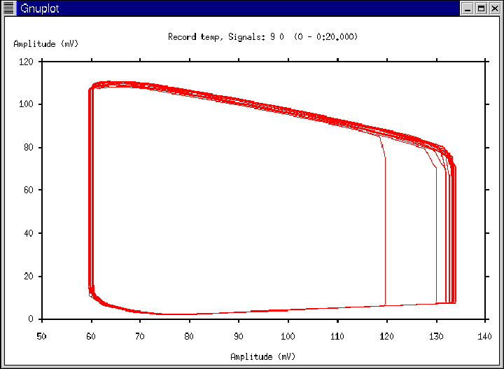
Figure 11: Gnuplot window generated according to Ex. 2.

Ex. 3

• Desired Execution:
  • On-line display of systemic arterial pressure, heart rate, and instantaneous lung volume with annotations.
  • Fully controlled, fully perturbed (fixed-rate breathing), intact pulsatile heart and circulation with default parameter values.
• Required Steps:
  1. Copy file $DIR/bin/parameters.def to the current directory with the new file name parameters_3.
  2. Open the file parameters_3 with any text editor (e.g., emacs).
  3. Re-assign the following parameters: waveform: 1 15 26, baro: 3, dncm: 1, breathing: 1, dra: 1, and df: 1.
  4. Save the file parameters_3.
  5. Execute the following command at the Linux prompt:
     rcvsim parameters_3 foo3
• Execution Output:
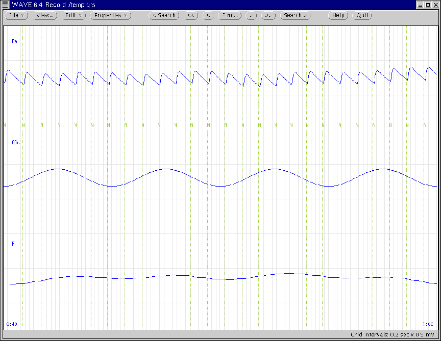
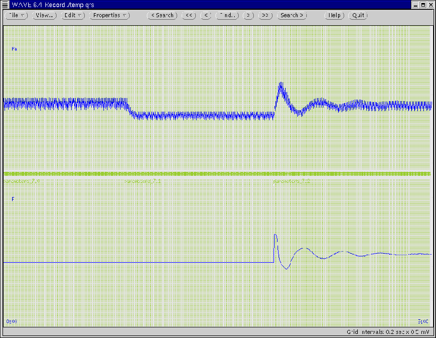
  • A WAVE window will appear and will automatically scroll through the simulated data with annotations. Figure 12 illustrates the window after one minute of data has been calculated. This process will terminate once 300 seconds of data have been simulated.
  • The following files will be created in the current directory: foo3.dat, foo3.qrs, foo3.hea, and parameters_3.0.

  

Figure 12: WAVE window generated according to Ex. 3 and Ex. 4.

Ex. 4

• Desired Execution:
  • Off-line display of systemic arterial pressure, heart rate, and instantaneous lung volume with annotations.
  • Fully controlled, fully perturbed (fixed-rate breathing), intact pulsatile heart and circulation with default parameter values.
• Required Steps:
  1. Copy file $DIR/bin/parameters.def to the current directory with the new file name parameters_4.
  2. Open the file parameters_4 with any text editor (e.g., emacs).
  3. Re-assign the following parameters: waveform: -1, baro: 3, dncm: 1, breathing: 1, dra: 1, and df: 1.
  4. Save the file parameters_4.
  5. Run the following command at the Linux prompt:
     rcvsim parameters_4 foo4
  6. Any time after the completion of the previous step, execute the following command at the Linux prompt:
     wave -r foo4 -s 1 15 26 -a qrs
  Or, if Ex. 3 have been previously implemented, then
  1. Execute the following command at the Linux prompt:
     wave -r foo3 -s 1 15 26 -a qrs
• Execution Output:
  • If Ex. 3 has not been previously implemented, then the following files will be created in the current directory: foo4.dat, foo4.qrs, foo4.hea, and parameters_4.0.
  • When the wave executable is implemented, a WAVE window will appear. The researcher may then use the arrow buttons at the top of the WAVE display system to scroll through the 300 seconds of generated waveforms with annotations. Figure 12 will appear after clicking the forward double arrow button twice or by directly running the wave executable with the following additional argument: -f 40.

Ex. 5

• Desired Execution:
  • On-line display of systemic arterial pressure and volume with annotations.
  • Uncontrolled, unperturbed, intact pulsatile heart and circulation initially with default parameter values.
  • On-line reduction in systemic arterial compliance by a factor of two.
• Required Steps:
  1. Copy file $DIR/bin/parameters.def to the current directory with the new file name parameters_5.
  2. Open the file parameters_5 with any text editor (e.g., emacs).
  3. Re-assign the following parameter: waveform: 1 10. Make sure all of the status parameters are assigned the numerical value of zero.
  4. Save the file parameters_5.
  5. Run the following command at the Linux prompt:
     rcvsim parameters_5 foo5
  6. Some time in the midst of the simulation, type ``p'' followed by $<$RETURN$>$ at standard input.
  7. Re-assign the the following parameter: Ca: 0.8.
  8. Save the file parameters_5.
  9. Type ``r'' followed by $<$RETURN$>$ at standard input.
• Execution Output:
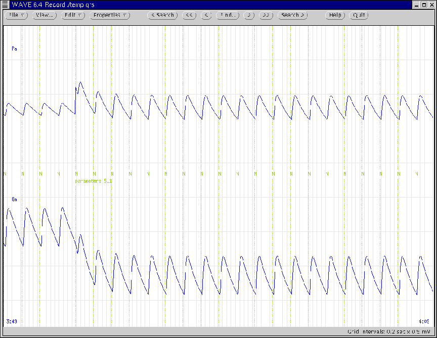
  • A WAVE window will appear and will automatically scroll through the simulated data with annotations. The automatic scrolling will stop once Step 6. is executed. (At this point, the researcher may scroll backwards with the the arrow buttons at the top of the WAVE display system.) After Steps 7.-9. are executed, automatic scrolling will resume until a total of 300 seconds of data have been calculated. Figure 13 illustrates the WAVE window during the time of reduction in systemic arterial compliance. Note that this reduction is annotated with the name of the saved parameter file. (Also note how systemic arterial volume is conserved through the instantaneous change in systemic arterial pressure.)
  • The following files will be created in the current directory: foo5.dat, foo5.qrs, foo5.hea, parameters_5.0, and parameters_5.1.

  

Figure 13: WAVE window generated according to Ex. 5.

Ex. 6

• Desired Execution:
  • On-line display of systemic arterial pressure, intrathoracic pressure, and instantaneous lung volume with annotations.
  • Uncontrolled, intact pulsatile heart and circulation initially with default parameter values perturbed by only fixed-rate breathing.
  • First, an on-line reduction in lung compliance by a factor of two. Then, an on-line, 500 ml step increase in the functional reserve volume of the lungs.
• Required Steps:
  1. Copy file $DIR/bin/parameters.def to the current directory with the new file name parameters_6.
  2. Open the file parameters_6 with any text editor (e.g., emacs).
  3. Re-assign the following parameters: waveform: 1 6 15 and breathing: 1.
  4. Save the file parameters_6.
  5. Run the following command at the Linux prompt:
     rcvsim parameters_6 foo6
  6. Some time in the midst of the simulation, type ``p'' followed by $<$RETURN$>$ at standard input.
  7. Re-assign the the following parameter: Clu: 126.25.
  8. Save the file parameters_6.
  9. Type ``r'' followed by $<$RETURN$>$ at standard input.
  10. At a subsequent time during the simulation, type ``p'' followed by $<$RETURN$>$ at standard input.
  11. Re-assign the the following parameter: Qfrs: 500.
  12. Save the file parameters_6.
  13. Type ``r'' followed by $<$RETURN$>$ at standard input.
• Execution Output:
  • A WAVE window will appear and will automatically scroll through the simulated data with annotations. The automatic scrolling will stop once Step 6. is executed. After Steps 7.-9. are executed, automatic scrolling will resume until Step 10. has been executed. When Steps 11.-13. are executed, the automatic scrolling will resume until a total of 300 seconds of data have been simulated. Figure 14 illustrates the WAVE window during the reduction in lung compliance. (Note that this reduction does not alter instantaneous lung volume; see Section 5.3.2). Figure 15 illustrates the WAVE window during the time of the step increase in the functional reserve volume of the lungs. (Note that the step increase occurs once the current respiratory cycle is complete.)
  • The following files will be created in the current directory: foo6.dat, foo6.qrs, foo6.hea, parameters_6.0, parameters_6.1, and parameters_6.2.
    

  

Figure 14: WAVE window generated according to the first parameter update of Ex. 6.

  

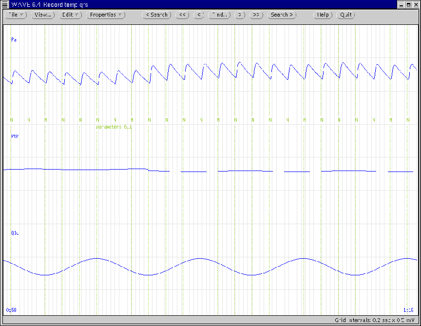Figure 15: WAVE window generated according to the second parameter update of Ex. 6.

Ex. 7

• Desired Execution:
  • On-line display of systemic arterial pressure and heart rate with annotations.
  • Uncontrolled, unperturbed, intact pulsatile heart and circulation initially with default parameter values.
  • First on-line hemmorhage of 500 ml. Then, on-line initiation of arterial and cardiopulmonary baroreflex control.
• Required Steps:
  1. Copy file $DIR/bin/parameters.def to the current directory with the new file name parameters_7.
  2. Open the file parameters_7 with any text editor (e.g., emacs).
  3. Re-assign the following parameters: waveform: 1 26, baro: 3, bgain: 0, again: 0, and pgain: 0.
  4. Save the file parameters_7.
  5. Run the following command at the Linux prompt:
     rcvsim parameters_7 foo7
  6. Some time in the midst of the simulation, type ``p'' followed by $<$RETURN$>$ at standard input.
  7. Re-assign the the following parameter: Qtot: 4500.
  8. Save the file parameters_7.
  9. Type ``r'' followed by $<$RETURN$>$ at standard input.
  10. At a subsequent time during the simulation, type ``p'' followed by $<$RETURN$>$ at standard input.
  11. Re-assign the the following parameters: bgain: 1, again: 1, and pgain: 1.
  12. Save the file parameters_7.
  13. Type ``r'' followed by $<$RETURN$>$ at standard input.
• Execution Output:
  • A WAVE window will appear and will automatically scroll through the simulated data with annotations. The automatic scrolling will stop once Step 6. is executed. After Steps 7.-9. are executed, automatic scrolling will resume until Step 10. has been executed. When Steps 11.-13. are executed, the automatic scrolling will resume until a total of 300 seconds of data have been simulated. Figure 16 illustrates the WAVE window once the simulation is complete. The Time variable of the WAVE window is set such that the waveforms over the entire simulation period may be viewed all at once. (Note how systemic arterial pressure has been returned to near normal values with the baroreflex systems.)
  • The following files will be created in the current directory: foo7.dat, foo7.qrs, foo7.hea, parameters_7.0, parameters_7.1, and parameters_7.2.

  

Figure 16: WAVE window generated according to Ex. 7 in which the time duration of the window has been expanded to illustrate the entire simulation period.

Ex. 8

• Desired Execution:
  • On-line display of a cardiac output curve.
  • On-line display of systemic arterial and venous pressure and left ventricle flow rate.
  • Uncontrolled, unperturbed, heart-lung unit preparation with default parameter values.
• Required Steps:
  1. Copy file $DIR/bin/parameters.def to the current directory with the new file name parameters_8.
  2. Open the file parameters_8 with any text editor (e.g., emacs).
  3. Re-assign the following parameters: time: 1000, waveform: 1 2 17, preparation: 1, Pas: 1000, and Pvs: 2.
  4. Save the file parameters_8.
  5. Run the following command at the Linux prompt:
     rcvsim parameters_8 foo8
• Execution Output:
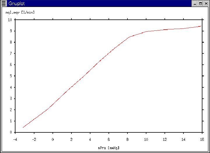
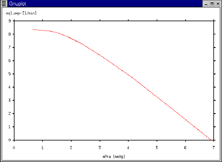
  • A WAVE window will appear and will automatically scroll through the simulated data as they are being calculated until the entire cardiac output curve has been measured. Figure 17 illustrates the WAVE window at the end of the simulation. (As is always the case with viewing waveforms on-line, the parameter values may be updated prior to simulation termination, if desired.)
  • Then, the Gnuplot window of Figure 18 will appear immediately following the calculation of the entire cardiac output curve.
  • The following files will be created in the current directory: foo8.dat, foo8.qrs, foo8.hea, foo8.txt and parameters_8.0.

  

Figure 17: WAVE window generated according to Ex. 8.

  

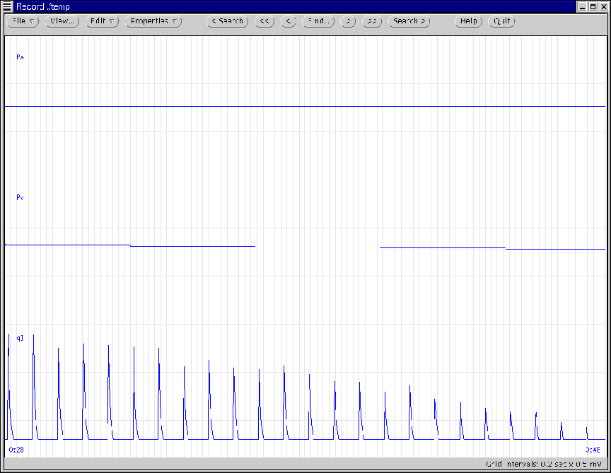Figure 18: Gnuplot window generated according to Ex. 8, Ex. 10, and Ex. 11.

Ex. 9

• Desired Execution:
  • On-line display of a venous return curve.
  • Uncontrolled, unperturbed, systemic circulation preparation with default parameter values.
• Required Steps:
  1. Copy file $DIR/bin/parameters.def to the current directory with the new file name parameters_9.
  2. Open the file parameters_9 with any text editor (e.g., emacs).
  3. Re-assign the following parameters: time: 1000, waveform: -1, preparation: 2, and Crds: 5.
  4. Save the file parameters_9.
  5. Run the following command at the Linux prompt:
     rcvsim parameters_9 foo9
• Execution Output:
  • The Gnuplot window of Figure 19 will appear immediately following the calculation of the entire venous return curve.
  • The following files will be created in the current directory: foo9.dat, foo9.qrs, foo9.hea, foo9.txt and parameters_9.0.

  

Figure 19: Gnuplot window generated according to Ex. 9.

Ex. 10

• Desired Execution:
  • On-line display of multiple cardiac output and venous return curves.
  • Uncontrolled, unperturbed, heart-lung unit and systemic circulation preparations with default parameter values and after a 25% increase in systemic arterial resistance, mean systemic pressure, heart rate, and contractility.
• Required Steps:
  1. Copy file $DIR/bin/parameters.def to the current directory with the new file name parameters_10.
  2. Open the file parameters_10 with any text editor (e.g., emacs).
  3. Re-assign the following parameters: time: 1000, waveform: -1, preparation: 1, Pas: 1000, and Pvs: 2.
  4. Save the file parameters_10.
  5. Run the following command at the Linux prompt:
     rcvsim parameters_10 foo10a
  6. Once the simulation is complete, re-assign the following parameters: numerics: 1, preparation: 2, and Crds: 5.
  7. Save the file parameters_10.
  8. Run the following command at the Linux prompt:
     rcvsim parameters_10 foo10b
  9. Once the simulation is complete, re-assign the following parameters: Ra: 1.25 and Pms: 8.625.
  10. Save the file parameters_10.
  11. Run the following command at the Linux prompt:
      rcvsim parameters_10 foo10c
  12. Once the simulation is complete, re-assign the following parameters: preparation: 1, Cls: 0.3, Crs: 0.9, and F: 1.5.
  13. Save the file parameters_10.
  14. Run the following command at the Linux prompt:
      rcvsim parameters_10 foo10d
• Execution Output:
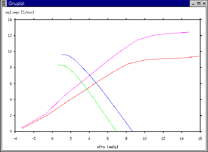
  • A total of four Gnuplot windows will be displayed beginning with a window displaying a single cardiac output curve (see Figure 18); then a window displaying the previous cardiac output curve with a venous return curve; followed by a window displaying these two previous curves with another venous return curve which is enhanced; and ending with a window displaying each of these three curves and an additional enhanced cardiac output curve (see Figure 20). (Note the increase in average cardiac output that occurs due to the enhancement of the curves.) Each of the four windows will appear immediately after the completion of each of the four rcvsim executions (Steps 5., 8., 11., 14.).
  • The following files will be created in the current directory: foo10a.dat, foo10a.qrs, foo10a.hea, foo10a.txt, foo10b.dat, foo10b.qrs, foo10b.hea, foo10b.txt, foo10c.dat, foo10c.qrs, foo10c.hea, foo10c.txt, foo10d.dat, foo10d.qrs, foo10d.hea, foo10d.txt and parameters_10.0.
    

  

Figure 20: Gnuplot window generated according to Ex. 10 and Ex. 11.

Ex. 11

• Desired Execution:
  • Off-line display of the cardiac output and venous return curves generated from Ex. 10.
• Required Steps:
  1. Change directory to that which contains the simulated data of Ex. 10.
  2. Run gnuplot at the Linux prompt.
  3. At the Gnuplot prompt, enter the following commands:
     set tics out
     set xlabel 'mPra [mmHg]'
     set ylabel 'mql,mqv [l/min]'
     plot 'foo10a.txt' using 1:2 notitle with lines
     replot 'foo10b.txt' using 1:2 notitle with lines
     replot 'foo10c.txt' using 1:2 notitle with lines
     replot 'foo10d.txt' using 1:2 notitle with lines
     (Note that the plot command is similar to numerics: 0, while the replot command is analogous to numerics: 1.)
• Execution Output:
  • A total of four Gnuplot windows will be displayed beginning with a window displaying a single cardiac output curve (see Figure 18); then a window displaying the previous cardiac output curve with a venous return curve; followed by a window displaying these two previous curves with another venous return curve which is enhanced; and ending with a window displaying each of these three curves and an additional enhanced cardiac output curve (see Figure 20).

Ex. 12

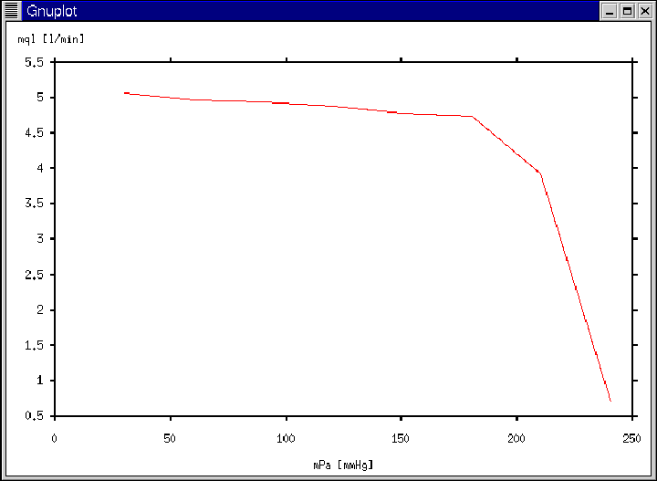
• Desired Execution:
  • On-line display of average cardiac output as a function of average systemic arterial pressure.
  • Uncontrolled, unperturbed, heart-lung unit preparation with default parameter values.
• Required Steps:
  1. Copy file $DIR/bin/parameters.def to the current directory with the new file name parameters_12.
  2. Open the file parameters_12 with any text editor (e.g., emacs).
  3. Re-assign the following parameters: time: 1000, waveform: -1, numerics: 2, preparation: 1, Pas: 30, and Pvs: 100.
  4. Save the file parameters_12.
  5. Run the following command at the Linux prompt:
     rcvsim parameters_12 foo12
• Execution Output:
  • The Gnuplot window of Figure 21 will appear immediately following the calculation of the entire curve.
  • The following files will be created in the current directory: foo12.dat, foo12.qrs, foo12.hea, foo12.txt and parameters_12.0.

  

Figure 21: Gnuplot window generated according to Ex. 12 and Ex. 13.

Ex. 13

• Desired Execution:
  • Off-line display of the curve of average cardiac output as a function of average systemic arterial pressure generated from Ex. 12.
• Required Steps:
  1. Change directory to that which contains the simulated data of Ex. 12.
  2. Run gnuplot at the Linux prompt.
  3. At the Gnuplot prompt, enter the following commands:
     set tics out
     set xlabel 'mPa [mmHg]'
     set ylabel 'mql [l/min]'
     plot 'foo12.txt' using 3:2 notitle with lines
     
• Execution Output:
  • The Gnuplot window of Figure 21 will again appear.