


Next: Other Models
Up: manual
Previous: Viewing Examples
A Research Example
The human cardiovascular model upon which RCVSIM is based was
originally constructed in order to advance research in the general
area of beat-to-beat hemodynamic variability [4,,8]. The RCVSIM software enhances
the potential of the original human cardiovascular model in
facilitating cardiovascular research by making the model more user
friendly and compatible with the open-source software provided by
PhysioNet. By further disseminating RCVSIM to the
cardiovascular research community through PhysioNet, researchers may
conveniently utilize the computational model to complement their
studies with the experimental data sets available on PhysioNet. For
example, RCVSIM has been previously utilized to develop an
algorithm for monitoring systemic arterial resistance from only a
peripheral arterial pressure waveforms which was subsequently
validated with data from the MIMIC database on PhysioNet
[4]. Another research example which illustrates how
RCVSIM may be utilized in conjunction with the open-source
software and experimental data sets of PhysioNet in order to improve
the accuracy of the model, and thus possibly physiologic
understanding, is provided below.
The default or nominal parameter values of the human cardiovascular
model are set such that the power spectra of the simulated
beat-to-beat hemodynamic variability resembles power spectra measured
from a group of normal humans in the standing posture
[4,5]. The objective of the research
example here is to determine a set of parameter values which permit
the model to generate a realistic supine posture, heart rate
power spectrum. In order to address this objective, it is necessary
to obtain experimental data sets to define what is realistic and
software to compute the heart rate power spectrum - both of which are
available from PhysioNet. The specific steps which were implemented
to achieve the research objective are given below.
- Establish realistic supine posture, heart rate power spectrum.
- Visit the following web page:
http://www.physionet.org/physiobank/database/meditation/data/
which houses Exaggerated Heart Rate Oscillations During two
Meditation Techniques: Data.
- Download the data in the metronomic breathing group from the
bottom of this web page - M#.hea and M#.qrs, where #
ranges from 1 to 14. (These data provide the qrs times of 14
volunteer subjects in the supine posture breathing at a fixed-rate
of 0.25 Hz.)
- Calculate an instantaneous heart rate tachogram from the qrs
times for each subject by executing the following command at the
Linux prompt (14 times):
tach -r M# -a qrs -f  hr#
hr#
(Note that tach is open-source software provided by PhysioNet. Type
tach -h at the Linux prompt for help.)
- Calculate the maximum entropy power spectrum of the
instantaneous heart rate tachogram for each subject by executing the
following command at the Linux prompt (14 times):
memse -f 2 -Z -o 15 hr# phr#
(Note that memse is open-source software provided by PhysioNet.
Type memse -h at the Linux prompt for help. The generated
files phr# are two-column, ASCII format files in which the
first column represents frequencies and the second column represents
the corresponding power spectral densities.)
- Average the power spectra over the 14 subjects and write the
averaged spectra to a two-column ASCII file called avephr (by
writing a simple program or using any pre-existing software such as
MATLAB).
- Plot the averaged power spectrum by executing the following
command at the Linux prompt:
plot2d avephr 0 1
(Note that plot2d, which is a simple program that controls Gnuplot,
is open-source software provided by PhysioNet. Type plot2d -h
at the Linux prompt for help.)
- Determine model parameter values which permit the model and
averaged, experimental heart rate power spectra to match.
- Copy file $DIR/bin/parameters.def to the current
directory with the new file name parameters_r.
- Open the file parameters_r with any text editor (e.g.,
emacs).
- Re-assign the following parameters: waveform: -1, baro: 3, dncm: 1, breathing: 1, dra: 1, df: 1, Tr: 4, and Qt: 430. (Since accompanying
experimental respiratory data is not available, the last parameter
is arbitrarily set such that the alveolar ventilation rate is 70
ml/s.)
- Save the file parameters_r.
- Execute the following commands at the Linux prompt:
rcvsim parameters_r foor
tach -r foor -a qrs -f hrsim
memse -f 2 -Z -o 15 hrsim phrsim
plot2d phrsim 0 1
- If this plot matches the experimental plot above, then the
research objective has been achieved. Otherwise, re-assign the
following parameters: bgain, again, pgain, stdwr, and stdwf, and repeat the steps above beginning with
Step (d). (Note that these five parameters have been identified
based on a priori knowledge of the physiologic differences between
supine and standing postures.)
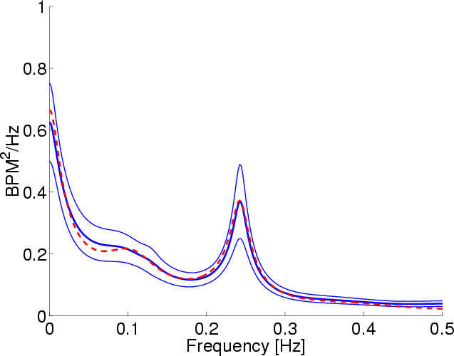
When the values assigned to the parameters of Step (f) are set as
follows: bgain: 0.5, again: 0.5, pgain: 1, stdwr: 0.04, and stdwf: 0.175, the averaged experimental and
model supine posture, heart rate power spectra match (see
Figure 22). As expected, the parameter changes from
the standing posture to supine posture reflected a shift in autonomic
balance favoring the parasympathetic nervous system. Interestingly, a
further comparison of these parameter values with the nominal values
suggests that the posture peak in humans ( 0.1 Hz
[10]; present in the model with default parameter
values) could be due to both a system resonance which is established
by increased sympathetic nervous activity as well as increased
fluctuations in local vascular resistance beds which may be due to
increased leg muscle activity.
0.1 Hz
[10]; present in the model with default parameter
values) could be due to both a system resonance which is established
by increased sympathetic nervous activity as well as increased
fluctuations in local vascular resistance beds which may be due to
increased leg muscle activity.
Figure 22:
Model (red) and experimental (blue) supine posture, heart
rate power spectra at fixed-rate breathing of 0.25 Hz. The dark
blue line is the average spectrum computed from 14 volunteers,
while the two lighter blue lines are the corresponding 95%
confidence intervals. See text for additional details.
 |
Next: Other Models
Up: manual
Previous: Viewing Examples
Ramakrishna Mukkamala (rama@egr.msu.edu)
2004-02-03