Method

Using a modified Fourier filtering method[63], we generate stationary uncorrelated, correlated, and anti-correlated signals $u(i)$ ( $i=1,2,3,...,N_{\mbox{\scriptsize max}}$) with a standard deviation $\sigma =1$. This method consists of the following steps:
(a) First, we generate an uncorrelated and Gaussian distributed sequence $\eta(i)$ and calculate the Fourier transform coefficients $\eta(q)$.
(b) The desired signal $u(i)$ must exhibit correlations, which are defined by the form of the power spectrum

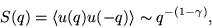$$S(q)=\langle u(q)u(-q) \rangle \sim q^{-(1-\gamma)},$$ (1)

where $u(q$) are the Fourier transform coefficients of $u(i)$ and $\gamma$ is the correlation exponent. Thus, we generate $u(q$) using the following transformation:

$$u(q)=[S(q)]^{1/2}\eta(q),$$ (2)

where $S(q)$ is the desired power spectrum in Eq. (1).
(c) We calculate the inverse Fourier transform of $u(q$) to obtain $u(i)$.
We use the stationary correlated signal $u(i)$ to generate signals with different types of nonstationarity and apply the DFA method[3] to quantify correlations in these nonstationary signals.
Next, we briefly introduce the DFA method, which involves the following steps[3]:
(i) Starting with a correlated signal $u(i)$, where $i=1,..,N_{max}$ and $N_{max}$ is the length of the signal, we first integrate the signal $u(i)$ and obtain $y(k)\equiv\sum_{i=1}^{k}[u(i)-\langle u \rangle]$, where $\langle u \rangle$ is the mean.
(ii) The integrated signal $y(k)$ is divided into boxes of equal length $n$.
(iii) In each box of length $n$, we fit $y(k)$, using a polynomial function of order $\ell$ which represents the trend in that box. The $y$ coordinate of the fit line in each box is denoted by $y_n(k)$ (see Fig. 1, where linear fit is used). Since we use a polynomial fit of order $\ell$, we denote the algorithm as DFA-$\ell$.

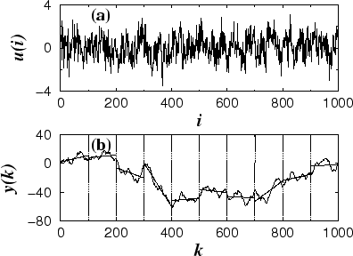
Figure 1: (a) The correlated signal $u(i)$. (b) The integrated signal: $y(k)=\sum_{i=1}^k[u(i)-\langle u \rangle]$. The vertical dotted lines indicate a box of size $n=100$, the solid straight lines segments are the estimated linear ``trend'' in each box by least-squares fit.

(iv) The integrated signal $y(k)$ is detrended by subtracting the local trend $y_n(k)$ in each box of length $n$.
(v) For a given box size $n$, the root mean-square (r.m.s.) fluctuation for this integrated and detrended signal is calculated:

$$F(n)\equiv\sqrt{{1\over {N_{max}}}\sum_{k=1}^{N_{max}}[y(k)-y_n(k)]^2}.$$ (3)

(vi) The above computation is repeated for a broad range of scales (box sizes $n$) to provide a relationship between $F(n)$ and the box size $n$.
A power-law relation between the average root-mean-square fluctuation function $F(n)$ and the box size $n$ indicates the presence of scaling: $F(n) \sim n^{\alpha}$. The fluctuations can be characterized by a scaling exponent $\alpha$, a self-similarity parameter which represents the long-range power-law correlation properties of the signal. If $\alpha =0.5$, there is no correlation and the signal is uncorrelated (white noise); if $\alpha <0.5$, the signal is anti-correlated; if $\alpha >0.5$, the signal is correlated[64].

We note that for anti-correlated signals, the scaling exponent obtained from the DFA method overestimates the true correlations at small scales[61]. To avoid this problem, one needs first to integrate the original anti-correlated signal and then apply the DFA method[61]. The correct scaling exponent can thus be obtained from the relation between $n$ and $F(n)/n$ [instead of $F(n)$]. In the following sections, we first integrate the signals under consideration, then apply DFA-2 to remove linear trends in these integrated signals. In order to provide a more accurate estimate of $F(n)$, the largest box size $n$ we use is $N_{max}/10$, where $N_{max}$ is the total number of points in the signal.

We compare the results of the DFA method obtained from the nonstationary signals with those obtained from the stationary signal $u(i)$ and examine how the scaling properties of a detrended fluctuation function $F(n)$ change when introducing different types of nonstationarities.