Variability vs. Complexity is one in a series of PhysioNet tutorials. Its goal is to introduce students and trainees to the study of complex variability, especially in the context of physiology and medicine. We invite comments and feedback from readers.
If you haven't found something strange during the day, it hasn't been much of a day.
—John Archibald Wheeler (1911-2008), eminent American physicist who coined the term "black hole"
Now my own suspicion is that the Universe is not only queerer than we suppose, but queerer than we can suppose.
—JBS Haldane (1892-1964), British geneticist
Variety's the very spice of life,
That gives it all its flavour.
—William Cowper (1731-1800), English poet
1.1 Variable Meanings of Variability
The term variability is used in many different contexts, both in everyday speech and in technical investigations. Scientists use the term in a wide number (variety) of ways, ranging from descriptions of genetic differences and phenotypic variations to characterizations of the ways patterns change over time. These temporal variations, or dynamics, may occur over spans ranging from milliseconds or less, to years or more. The concepts of hereditable variability and natural selection are, of course, foundational pillars of Darwin’s theory of evolution.
In other domains, variability at differing time scales is encountered in discussions of climate change, economic forecasting, and crisis management, in which long-term trends may be obscured by short-term fluctuations.
On a more physiological level, analysis and understanding of the way that our vital signs fluctuate may offer new approaches to medical diagnosis and therapeutics. To foster these translational activities, PhysioNet includes an extensive collection of tutorial material, computational tools, and datasets related to physiological dynamics, an important example of which is heart rate variability (HRV). This term refers to the analysis of beat-to-beat changes in cardiac interbeat intervals for extraction of basic and clinical information.
HRV analysis is one of the most widely-studied applications of dynamics to human physiology. A search for "heart rate variability" in PubMed yielded over 9000 results as of January 2012. A closely related area has been referred to as heart rate characteristics analysis, focused on measurement of beat-to-beat changes that occur in conjunction with neonatal sepsis [Griffin 2007, Moorman 2011].
1.2 Approaching a Definition of Complexity
A concept that is closely connected to that of variability is complexity. Indeed, one question is whether the connection is so close that the two terms are actually synonymous [Bar-Yam 1997]. If that were the case, it would substantially truncate this tutorial (at this sentence!). In contemporary science, however, the term complexity has a meaning that is qualitatively and quantitatively distinguishable from traditional concepts and metrics of variability.
To avoid any possible misunderstanding, let us first make it clear that complexity has nothing to do with being complicated, nor with numbers containing imaginary components.
Complex variability is synonymous with complexity, and it hints at the distinction between complexity and variability. Things that exhibit complexity (complex variability) also exhibit variability, but not everything that varies exhibits complexity.
Perhaps, we can begin to converge on a common understanding of what it means to say that a time series exhibits variability, and what it means to say that it exhibits complex variability. At the very least, we can try to develop a framework for understanding where expert disagreements lie and what scientific agenda might be followed to resolve them.
Every presentation has a certain bias or slant, sometimes more diplomatically called a point of view. Our agenda is to convey and provide support for the following two points of view:
- Complexity is different from variability.
- The concept of complex variability can be usefully applied to the study of physiologic time series.
As part of this brief tutorial, we will give an overview of some computational approaches that may be useful in deciding whether a time series is complex and whether the output of some model or simulation captures fundamental properties of real-world data.
1.3 Time Series, Signals, Samples, and Conventional Statistical Measures of Variability
A time series, as implied by the name, is a sequence of values that represent the time evolution of a given variable. In this tutorial, we use the word signal interchangeably with time series. The word signal has other meanings that include messages, information (as distinct from noise), and continuously changing quantities; we do not use "signal" in any of these senses in this tutorial. Often, we (and others) tend to use "signal" for densely-sampled time series that represent continuous processes well, reserving "time series" for sparsely or unevenly sampled sequences of measurements. The individual measurements or observations that comprise a time series or signal are samples (another word with multiple meanings, used only in this sense below).
Familiar physiologic variables that may be presented as time series include heart rate, breathing rate and volume, cardiac output, arterial oxygen saturation, pulmonary and systemic blood pressures (systolic, diastolic and mean values), serum glucose, and so forth.

Figure 1. Heart rate time series from a healthy subject. Note the irregular pattern of fluctuations with changes in mean and variance (nonstationarity).
The most informative biomedical datasets are usually those that include uninterrupted recordings of multiple physiologic signals collected under well-characterized, clinically relevant conditions.
Statistically, the amount of variability in individual or group behavior is typically probed with measures related to the sample variance, including the standard deviation (SD), the standard error of the mean (SE or SEM), and the coefficient of variation (CV). In scientific presentations, both formal and informal, and for publication, you will usually see the variability summarized with a type of bar graph that typically gives the mean value, plus/minus the SD or SEM.
Another graphical data summary that you will likely encounter in the biomedical literature is the box plot (also referred to as the box and whisker plot). This graph classically shows 5 values per dataset: 1) the minimum value; 2) the lower quartile (the value below which contains 25% of the data); 3) the median (middle value); 4) the upper quartile (the value above which contains 25% of the data), and 5) the maximum value. These types of plots have the advantage that they give a fuller descriptive summary of the data than the classic mean +/- SD or SEM summaries and a better sense of outliers.
Students need to be aware that even the most elaborate box and whisker plots have inherent limitations. These plots do not give information about the temporal order of the data points. Therefore, different time series can have the same box plot as long as their histogram/distribution is the same. As we will see, however, the order in which the different values appear contains information about nature of the dynamics.
Consider the two following heart rate time series. The datasets are derived from recordings of two different individuals during sleep. One is healthy; the other has an important medical condition called obstructive sleep apnea in which intermittent collapse of the upper airway leads to cessation of effective breathing.
The two heart rate sequences have nearly identical mean values and variances for the given observation period (about 15 min). Despite their statistical commonalities, the two time series look different to visual inspection.

Figure 2. Two heart rate time series with identical means and variances. One is from a healthy subject; the other from a subject with sleep apnea. Which one is more complex? Which signal is from which subject? (Answers below.)
For a discussion of obstructive sleep apnea and how to identify evidence of it in cases such as those illustrated above, see Detection of Obstructive Sleep Apnea from Cardiac Interbeat Interval Time Series.
1.4 What is Complex Variability, and Can it be Measured?
One point of agreement about complexity, and perhaps the only point of consensus, is that no formal definition of this term exists. Try polling scientists representing different or even the same communities. You will encounter a considerable range of variable views, all strongly held and some leading to contradictory conclusions, even when looking at the same data sets.
Intuition suggests that "simple" (not particularly complex) sequences of observations are readily comprehended: they can be described concisely, they contain no surprises, and their information content is low. Conversely, complex series are not easy to understand completely: they are full of surprises, they require lengthy descriptions, and their information content is high. If we remove one sample from a time series, its value can be estimated using the information contained in the rest of the series; this process will be easy for a simple series, and more difficult (but still possible) for a complex series. More precisely, we can say that the expected squared error of our estimate will be less than the variance of the series using an estimator that makes appropriate use of information obtained from the other samples.
What is the complexity of white noise, a time series in which the samples are random and uncorrelated? Here, the problem of estimating a missing sample is neither easy nor difficult; indeed, it is not possible, because (by definition) there is no information in the remainder of the series that is at all relevant to the problem of estimating the missing value. Within the framework of our intuitive argument above, the complexity of white noise is undefined.
A useful clinical example of a signal with dynamics close to white noise is the short-term response of the ventricles during atrial fibrillation. Clinicians refer to this rhythm as irregularly irregular, a somewhat cumbersome way of saying random appearing. Of interest, atrial fibrillation is one of the most common cardiac arrhythmias, especially prevalent with aging and a variety of different cardiac syndromes (e.g., high blood pressure or cardiomyopathy) and represents a mal-adaptive (non-complex) pathophysiologic state.

Figure 3. Electrocardiogram (ECG) rhythm strip (about 7.6 s) showing atrial fibrillation. Note the irregular, rapid ventricular (QRS) response. The interbeat interval time series of such a signal has a relatively high entropy value, although the signal itself represents a loss of physiologic information.
One family of approaches to measuring complexity, derived from information theory, is based on quantifying the degree of compressibility of signals. The first and best-known of these approaches is algorithmic entropy. The fundamental idea underlying this family of approaches is that simple sequences can be described concisely, and complex sequences cannot; hence a method for producing a compact description of a sequence can be used to estimate its complexity as the ratio of the size of the size of its description (compressed representation) to its original size. Measurements derived using these approaches suggest that the most compressible signals (such as constant or strictly periodic signals) are the least complex, which is consistent with our intuitive framework for complexity. At the other extreme, however, the only signals that are totally incompressible are random uncorrelated signals (white noise), and compressibility-based approaches suggest that such signals are the most complex, a conclusion which many (including the authors of this tutorial) consider to be a serious weakness of these approaches.
A closely related idea, motivated by the observation that unpredictability (entropy) frequently reflects complexity, has led to the use of entropy-based measures such as ApEn and SampEn as surrogate measures for complexity. Although such measures can be useful in some cases (such as in characterizing the important difference between series A and B in Figure 2 above), they are not universally applicable, since an increase in the entropy (disorder) of a system is not necessarily always associated with an increase in its complexity.
As an example of the flaws of both compressibility-based and entropy-based measures, compare the time series of musical notes in Mozart’s Jupiter symphony with the "music" you might generate by shuffling those notes. Characteristics of the symphony such as its harmonic, rhythmic, melodic, and contrapuntal structures are all representative of information content over time scales from beats to measures to phrases to symphonic movements — and all of this information content is absent from the shuffled-note series. Thus it should be clear that Mozart's series of notes has a greater information content and is more complex than the shuffled-note series, but methods such as algorithmic entropy, ApEn, and SampEn point to the contrary conclusion, since the shuffled series is less compressible and less predictable than the original.
This finding raises the question: can entropy-based methods be adapted to quantify complex variability?
One approach is to test whether a time series contains information on multiple time scales, an idea that is the basis of multiscale entropy (MSE) [Costa 2002], which is the subject of a separate tutorial. This approach is motivated by the observation that complex signals encode information over multiple time scales, whereas uncorrelated random signals or very periodic signals do not. The multiscale entropy algorithm was developed to help distinguish uncorrelated random signals from more complex (information-rich) signals (e.g. 1/f noise).
The authors of this tutorial and colleagues have adopted a framework according to which random uncorrelated series of samples are among the least complex signals, and those with so-called long-range correlations are among the most complex. As central facets of this framework as applied to biologic systems, we suggest three, inter-related working hypotheses:
- The degree of complexity of a biologic/physiologic signal recorded under free-running conditions (baseline) reflects the complexity of the underlying dynamical system.
- Complexity is closely related to adaptability. The more adaptive the individual organism, the more complex the signals it produces are likely to be.
- Complexity degrades with pathology and aging (theory of decomplexification with disease). In the latter context, the loss of complexity is most apparent in subjects with advanced (pathologic) aging, referred to as the frailty syndrome.
Why would physiologic signals be so complex? One speculation is that complex fluctuations result from the activity of control mechanisms responding to internal and external changes in biologic parameters and the interactions (cross-talk) among them. In contrast random outputs result from degraded control mechanisms and/or the breakdown of the coupling among them. In the same line of reasoning, very periodic signals, such as series B in Figure 2, may arise from a variety of pathologic conditions including excessive synchronization/coupling between control mechanisms, drop out of some control loops, and/or excessive delays that have been shown to induce periodic oscillators [Glass 1988].
So far, our discussion has focused on the dynamics of individual organisms. A question worth discussing is whether these hypotheses can be generalized to macro-systems of interacting individuals (from cell to society levels). One conjecture is that they do and that loss of complexity is a marker, not just of impaired health or functionality of cells, organ systems and individuals, but also of ecosystems and perhaps even of human social systems that are at risk of extinction.
2 Complexity in the Physical World
In the physical (non-living) world, some of the most complex signals arise from turbulent flows. Indeed, turbulent dynamics, as seen in ocean waves, waterfalls, and jet engine plumes, create an astonishing array of spatial and temporal structures. These dynamics present some of the most daunting, unsolved challenges in physics and mathematics. Surprisingly, this class of dynamics appears to have connections to the types of multiscale structural and functional properties that seem essential to life itself. An exciting and likely prospect is that concepts and tools from statistical physics and applied mathematics that are used in the analysis of turbulent flows can be adapted to gain insight into mechanisms underlying biologic fluctuations. Equally exciting is the possibility that the challenges posed by analyzing biologic systems will foster the development of new mathematical approaches, which will in turn help illuminate the physiologic world within us and the natural, sometimes turbulent world we inhabit [Ivanov 1999].
3 Some Ingredients of Biologic and Physiologic Complexity
What are the ingredients that help identify a signal as complex? In biology in general, and human physiology in particular, complex signals generated by healthy organisms typically manifest at least one, and usually an ensemble, of the following dynamical properties: (1) nonlinearity––the relationships among components are not additive, so small perturbations can cause large effects; (2) nonstationarity––the statistical properties of the system’s output change with time; (3) time irreversibility or asymmetry––systems dissipate energy as they operate far-from-equilibrium and display an arrow of time signature; (4) multiscale variability––systems exhibit patterns in space and time over a broad range of scales. Further, this multiscale spatio-temporal variability may be fractal-like. An example of a physiologic signal that displays all four of these attributes simultaneously is the healthy human heartbeat (or, inversely, the cardiac interbeat interval) obtained at rest or with minimal activity (e.g., series A in Figure 2).
We will briefly review these properties.
3.1 Linearity vs. Nonlinearity
The simplest definition of a nonlinear system is that the system (or its output) is literally not linear. Anything that fails criteria for linearity is nonlinear [Kaplan 1995, Goldberger 2006]. Linear systems are easily recognized since their output (y) is controlled by the input according to straightforward equations of the type y = mx + b. One classic example is given by Ohm’s law: V = IR, where the voltage (V) in a circuit will vary (over some range) linearly with current (I), provided the resistance (R) is held constant.
Two key properties of linear systems are proportionality and superposition. Proportionality indicates that the output bears a straight line relationship to the input. The superposition principle applies when the behavior of systems composed of multiple sub-components can be fully understood and predicted by dissecting out these components and figuring out their individual input-output relationships. The overall output will be a summation of these constituent parts. The components of a linear system literally add up. Therefore, linear systems can be fully analyzed or modeled using a reductionist (dissective) strategy [Strogatz 1994, Buchman 2002].
In contrast, nonlinear systems defy comprehensive understanding by a classic reductionist approach. Even the simplest nonlinear systems will foil the criteria of proportionality and superposition. A classic example of a nonlinear system that is deceptive in its simple appearance is the logistic equation:
which, for the study of biologic population growth, can be rewritten as:
Equation (2) is called the quadratic recurrence equation.
The nonlinearity arises from the quadratic term (xn2). The simple-in-form logistic equation has inspired a large body of research and is the subject of a famous and highly readable 1976 paper in Nature by the eminent biomathematician, Sir Robert May [May 1976]. He urged that mentors introduce their students to this equation early in their mathematical, and one might add, biomedical, education since it "can be studied phenomenologically by iterating it on a calculator, or even by hand. It does not involve as much conceptual sophistication as does elementary calculus. Such study would greatly enrich the student’s intuition about nonlinear systems." High speed computing in contemporary computational devices makes numerical exploration of Equation 1 and its variants even more feasible.
If you calculate xn for a range of values of the parameter a, you will generate time series which exhibit a number of very different patterns. Some of these patterns are graphically shown below.

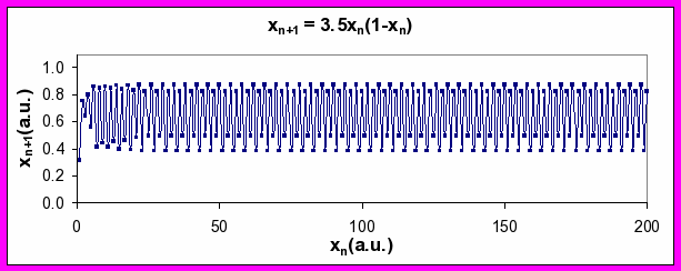

Figure 4. Series of xn values generated by Equation 2 for a values of 2.95 (top), 3.5 (middle), and 4 (bottom). Note period-doubling between top and middle plots, and transition to chaos between middle and bottom plots (see discussion below).
In the trivial cases when the parameter a (which can be interpreted as the food supply in an ecologic system), is set at 0 or xn is set at 0, the population becomes extinct. For a given range of x0 values, the output values xn will eventually settle down to straight-line type pattern, referred to as a steady state. Biologists would say that the population is stable.
An interesting phenomenon happens when you steadily increase the value of a, however. At a critical value, the output changes from a steady state and starts to oscillate with a frequency of k cycles per unit time. Further increases in a results in another abrupt change such that the frequency of oscillation goes to k/2 and then to k/4. In nonlinear systems, this abrupt jump from one characteristic frequency to a frequency half of the original (twice the wavelength) is referred to as period doubling bifurcation.
What happens as the parameter, a, is dialed up still higher? Something quite remarkable occurs. The output sequence goes from being very predictable (periodic: period-2, period-4 and period-8) to being very erratic. For a ≥ 4, the erratic output, which is effectively unpredictable beyond a limited number of time steps, is called nonlinear chaos. Interestingly, it arises from output from a system that is fully deterministic (no random terms).
Importantly, the mathematical definition of chaos has nothing to do with its everyday usage that indicates that things (personal, geopolitical or otherwise) are a mess. Detection of chaos in a time series can be done by measuring the largest Lyapunov exponent [Rosenstein 1993]. (Software for doing this is available in PhysioToolkit.) The application and interpretation of this method when applied to real-world data (like the human heart beat) has led to contradictory findings, however. Thus, the relevance of rigorously defined deterministic chaos to physiology, healthy or pathologic, remains an open question.
We also note that the qualitatively different dynamics demonstrated by the logistic equation under different parameter regimes present only a small subset of the much larger domain of field of nonlinear dynamics. Other examples of nonlinear dynamics include various wave phenomena, such as spiral waves, scroll waves and solitons, turbulence, nonlinear phase transitions, fractal geometric forms such as strange attractors that are created by the trajectories of chaotic processes, certain types of intermittent (pulsatile) behaviors, hysteresis, bistability and multistability (closely connected with time irreversibility), pacemaker synchronization/coupling and pacemaker annihilation phenomena, self-sustained oscillations, and so forth.
A final note to this section: Although deterministic chaos is only one example of nonlinear dynamics, the more general term chaos theory, particularly in the popular literature, has come to be virtually synonymous with nonlinear dynamics and with complexity theory. It should be understood that chaos theory does not imply chaotic dynamics as used above, and that a process that appears random may or may not reflect underlying chaotic dynamics.
3.2 Stationarity vs. Nonstationarity
If the statistical properties (mean, variance, and even higher moments) of a time series are approximately constant over some period of interest, the sequence is said to be stationary. Most biological signals, however, show changes in one or more statistical properties (e.g., mean, standard deviation, skewness and other higher moments, fractal properties, etc) over time, hence are nonstationary.
A commonly recognized type of nonstationarity arises from a slow change (drift or trend) of the time series’ mean value (your heart rate or blood pressure both tend to drift down during sleep). Another type arises from relative rapid transitions (such as the change in your heart rate and blood pressure when the alarm rings at 6:00 a.m.; or perhaps 11 a.m. if you are a grad student).
A sustained straight-line or sinusoidal output is clearly stationary. Virtually all biologic signals (except those from the sickest individuals over a sustained but obviously not very prolonged period) show some time-varying changes in one or more of their statistical properties, however, so when is it appropriate to consider a real-world time series stationary? Although a variety of stationarity tests have been proposed, it is not possible to avoid some arbitrariness in defining the criteria for judging stationarity. At a minimum, you need to specify the statistical properties you are referring to and the relevant time scale.
3.3 Multiscale Properties
An essential ingredient of living systems, even those on lower evolutionary rungs, is their spatio-temporal multiscale/hierarchical organization. From a structural (anatomic) view, biologic systems are composed of atoms and small molecules, macromolecules (proteins and glycoproteins, nucleic acids, etc), cellular components, cells, tissues, organs and then the entire organism (see our tutorial about Fractal Mechanisms in Neural Control). Further, each of us is part of large essential social networks that scale up from local to regional to global [Bar-Yam 1997, Buchman 2002].
A concept closely connected with multiscale spatio-temporal properties is fractality, as discussed in Exploring Patterns in Nature, another series of PhysioNet tutorials. The term fractal is most often associated with irregular objects that display a property called self-similarity or scale-invariance. Fractal forms are composed of subunits (and then sub-subunits, on so forth) that resemble (but are not necessarily identical to) the structure of the macroscopic object. In idealized (mathematical) models, this internal lookalike property holds across a wide range of scales. The biological world necessarily imposes upper and lower limits over which scale-free behavior applies [Goldberger 2006].
A large number of irregular structures in nature, such as branching trees and their root systems, natural coastlines, and rough-hewn mountain surfaces, exhibit fractal geometry. Complex anatomic structures such as the His-Purkinje conduction system in the heart and the tracheo-bronchial tree also display fractal-like features [Bassingthwaighte 1994]. These self-similar cardiopulmonary structures serve at least one, common fundamental physiologic function, namely rapid and efficient transport over multiscale, spatially distributed networks. Related to this function, the fractal tracheo-bronchial tree may also support mixing of gases in the distal airways [Tsuda 2002] and avalanche-like cascades in pulmonary inflation [Suki 1994].
With aging and pathology, fractal anatomic structures may show degradation in their structural complexity. Examples include loss of arborizing dendrites in aging neurons and vascular pruning characteristic of primary pulmonary hypertension [Goldberger 2002].
The fractal concept can be expanded from the analysis of irregular geometric forms that lack a characteristic (single) length scale to help assess complex processes that lack a single time scale. Fractal processes generate irregular fluctuations that are reminiscent of scale invariant structures having a branching or wrinkly appearance across multiple scales.
An important methodologic challenge is how to detect and quantify the fractal scaling and related correlation properties of physiologic time series, which are typically nonstationary. To help cope with the complication of nonstationarity in biological signals, Peng and colleagues introduced a fractal analysis method termed detrended fluctuation analysis (DFA).
3.4 Time Irreversibility (Asymmetry)
Another interesting, and perhaps fundamental, aspect of complex physiologic dynamics in health and life-threatening disease is illustrated in the two recordings in Figure 5. Shown are two time series plots similar to those presented earlier; except here we add an additional twist. Each time series is plotted in two directions. First, we show the recording in its usual time order, namely, present to future. Then we show the same record re-plotted with the arrow of time reversed, so it points from future to present. We can then visually assess what effect, if any, this experiment has on the dynamics.
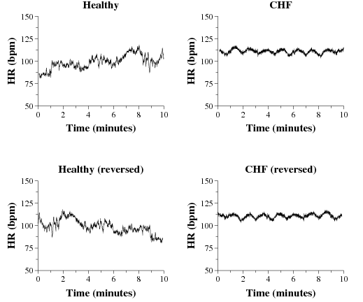
Figure 5. Ten-minute heart rate (HR) time series from a healthy volunteer (left) and from a patient with congestive heart failure (CHF, right). The lower panels contain the same data as in the upper panels, but time-reversed.
It is intriguing that, for the example shown here, the time reversal experiment has quite different effects on the two records. For the healthy subject’s data, reversing the arrow of time changes the appearance of the record completely. For the subject with severe heart disease, time reversal seems to have a less dramatic effect. The record appears to read the same way from right-to-left as it does from left-to-right. Time irreversibility seems to be largely lost in the pathologic state.
Time asymmetry (reversibility) is one of the most mysterious properties of complex systems. This property usually indicates a system that is in a non-equilibrium state. At equilibrium, time irreversibility is not seen. Time irreversibility is also closely related to a property called hysteresis. This term applies when the trajectory of a system in one direction and its reverse are different.
For the healthy heartbeat, the time asymmetry properties are of special interest since they are seen on multiple time scales. For a description of a computational algorithm to quantify the degree of time irreversibility of a time series, see [Costa 2008].
4 Do Complex Systems Always Generate Complex Signals?
An apparent paradox is that very linear (i.e., non-complex) signals may be generated from highly complex systems, including those responsible for healthy human physiology. An example, consider an artist’s ability to trace out a circle or straight line, or a tightrope walker’s uncanny ability to tread the straight and narrow with minimal tolerance for error. At peak exercise, even elite endurance athletes will show a marked loss of heart rate complexity.
Do such examples of linear-appearing outputs undermine the proposed link between complex systems and complex signals? The answer is no and the explanation relates to the close relationship between complexity and adaptiveness. Complex systems are capable of generating an extraordinary range of behaviors and outputs. The nature of these outputs, especially over relatively short time periods, is very much context- and task-dependent. If a system is complex and adaptive, it can shape its responses to the exigencies of the situation.
Of note is the finding that some of the most complex dynamics of the human heartbeat are observed under resting or relatively inactive conditions. This free-running or spontaneous complex variability is hypothesized to be an indicator of complexity reserve. If the individual is compelled to perform a task, this complexity reserve (akin to potential energy or information content) can be mobilized to produce a specific response from this reserve. In the case of heart rate dynamics, the loss of complex variability with exercise is followed by a relaxation (recovery) period in which slowing of the rate is accompanied by reappearance of complex variability.
In patients with severe congestive heart failure, a syndrome marked by inadequate cardiac output despite high ventricular filling (diastolic) pressures, heart rate complexity is reduced and the pattern of reduced variability, even at rest, resembles that of a healthy individual at the brink of exhaustion. For these patients, the number of different dynamical states (options) is diminished in comparison to those available to healthy subjects. Therefore, the difference in heart rate complexity between resting and active conditions is smaller for congestive heart failure patients than for healthy subjects.
5 Can Simple Systems Generate Complex Signals?
The answer to this question, of course, depends importantly on your definition of the word simple. If simple is taken to mean linear, then the answer is no. Linear systems cannot generate time series such as those observed in the healthy heartbeat with multiscale hysteresis (time reversibility) and multifractality. No mechanisms based on the superposition principle will yield these kinds of patterns.
What about simple-appearing nonlinear systems, such as the logistic equation or coupled systems of differential equations that yield strange attractors and chaotic behaviors [Strogatz 1994]? Clearly, the logistic equation (within certain parameter regimes) and differential equations used to generate mathematically chaotic outputs meet one or more of the criteria of complex behavior, though they do not have certain properties inherent in the complex biologic systems, including time irreversibility and long-range temporal correlations. Simple-appearing networks may also generate complex dynamics in particular parameter regimes [Amaral 2004].
The problem of simulating the healthy heartbeat was the subject of a PhysioNet/CinC Challenge, and the dataset from that challenge remains available for further study.
6 Can the Complexity of Already Complex Biologic Signals be Further Enhanced?
An intriguing question sometimes posed after discussions of the surprising complexity of healthy signals, such as cardiac interbeat interval time series, is: can you take such a signal and manipulate it such that is rendered even more complex? Or has nature evolved living systems such they generate the most complex signals (adaptive systems) possible? Since candidate signals possess fractal and multifractal features, in addition to multiscale time reversibility and multiscale entropy, they already are members of a class of elite or hyper-complex signals. Would a set of signals with statistically greater multifactality, higher asymmetry and higher multiscale entropy be more complex? How would one test that notion in an experimental way?
This task recalls the interchange between young Mozart and Emperor Joseph II in Peter Shaffer’s play and movie Amadeus:
Emperor Joseph II: My dear young man, don't take it too hard. Your work is ingenious. It's quality work. And there are simply too many notes, that's all. Just cut a few and it will be perfect.
Mozart: Which few did you have in mind, Majesty?
Caution is also warranted to the extent that complexity is not equivalent to a Rubik’s cube or Sudoku solution where everything neatly drops into place. More likely, biologic complexity arises as an emergent property, a type of phase transition, where the nonlinearities, nonstationarities, time irreversibility properties reflecting non-equilibrium dynamics, and the fractal/multifractal features have an "orchestral" organicity.
7 Complexity: Some Experimental Considerations
Designing experiments that involve the recording and analysis of complex physiologic signals raises some important considerations. Here we highlight selected aspects common to many different types of investigations. Of key overall importance is the need to be highly familiar with the data path: how were the signals obtained from the subject or experimental preparation, and how did they make their way to your computer or spreadsheet? In this sense, the data you analyze (from your own experiment or someone else’s) are like pieces of evidence in a forensic context.
Whenever possible, you should look at all of your data in graphical or other representational forms that allow you to get the lay of the land. This overview will help identify outliers that might indicate artifacts, an important source of spurious nonstationarity, as well as intrinsic changes in the patterns of the fluctuations that may be a clue to phase changes or bifurcation-type mechanisms.
Are you (or is the data acquisition/analysis system itself) doing any mathematical or other so-called data pre-processing maneuvers to filter, detrend or otherwise alter the rawest form of the signals? Care should be taken because often data acquisition and pre-processing procedures are carried out by algorithms embedded in proprietary devices in a black box fashion that makes it difficult or impossible to ascertain key aspects of the experimental recording and to recover the original signal.
Also from a technical point of view, deciding what constitutes adequate resolution and sufficient data length depends on the scientific question and underlying hypotheses. Suppose we had a physiologic time series sampled at 2 Hz. In this case, we would not be able to probe the dynamics on time scales smaller than one second, and therefore we could not assess the underlying control mechanisms operating below this threshold.
Real-world and synthetic data available at PhysioNet may help to resolve some of the current questions, prompt new ones, and lead to yet more sources of data, computational tools, and models.
8 Complexity in the Arts
Engineers and scientists are not the only members of communities who employ concepts of complexity. Observers and practitioners of the arts (including literature, music, painting and architecture) use the term "complexity" in ways, which, while not quantitative, may bring important insights to the tasks of the so-called hard sciences. The term "complexity" is sometimes used to convey the irreducible originality of great works of art. Paul Cézanne (1839-1906) reportedly observed, "I am progressing very slowly, for nature reveals herself to me in very complex forms; and the progress needed is incessant." (Cézanne is also reported to have said, memorably, "With an apple I will astonish Paris.") The French composer, Maurice Ravel (1875-1937), in his own words, aspired for his works to be "complex but not complicated."
Interested readers may find material on this theme at Heartsongs on one of the Resource’s affiliated websites.
As a related, interesting but digressive topic, some readers may also wish to explore and critically assess the expanding and provocative literature on the possible therapeutic uses of art in a number of major medical conditions, including Parkinson’s disease, dementia, stroke, pain management, and depression [Burton 2009].
9 Complexity vs. Variability: Working Conclusions
- The complexity of a time series is different from its variability or erratic-ness, as conventionally measured by the variance and related statistical metrics.
- Currently, no consensus definition of complexity exists.
- We explore an approach based on a biologically-motivated definition of complexity, in which the most complex signals are generated by organisms which are in their most adaptive (healthy) states.
- A sustained loss of complexity (decomplexification), under free-running (baseline or spontaneous) conditions, is observed in pathologic contexts, including disease and advanced aging (frailty) syndrome.
- We propose that the complexity of a signal relates to its structural richness and correlations across multiple time scales. Complex signals are information-rich. Two signals can have the same degree of statistical variability (i.e., the same global variance and coefficient of variation), but very different complexity properties.
- No single measure is sufficient to capture the properties of the most complex signals. Instead, an ensemble of measures is required, a type of statistical toolkit that allows you to probe signals of interest for different attributes.
- Such toolkits are necessary, but not sufficient, for measuring complexity since a comprehensive, mathematical approach to the simultaneous challenges posed by biologic signals is not yet developed.
- A partial list of the computational tools that may be useful includes measures of nonlinearity, nonstationarity, multiscale entropy (information), multiscale time irreversibility (asymmetry) and fractality/multifractality (see PhysioToolKit.)
Selected References
- [Griffin 2007]
- Griffin MP, Lake DE, O'Shea TM, Moorman JR.
Heart rate characteristics and clinical signs in neonatal sepsis.
Pediatr Res 2007;61:222-227.
- [Moorman 2011]
- Moorman JR, Carlo WA, Kattwinkel J, Schelonka RL, Porcelli PJ, Navarrete CT, Bancalari E, Aschner JL, Walker MW, Perez JA, Palmer C, Stukenborg GJ, Lake DE, O'Shea TM. Mortality reduction by heart rate characteristic monitoring in very low birth weight neonates: a randomized trial. J Pediatr 2011 Dec;159(6):900-6.e1.
- [Bar-Yam 1997]
- Bar-Yam Y. Dynamics of Complex Systems. Reading, Massachusetts: Perseus, 1997.
- [Costa 2002]
- Costa M, Goldberger AL, Peng CK. Multiscale entropy analysis of complex physiologic time series. Phys Rev Lett 2002;89:068102-1-4.
- [Glass 1988]
- Glass L, Mackey MC. From Clocks to Chaos: The Rhythms of Life. Princeton: University Press, 1988.
- [Ivanov 1999]
- Ivanov PC, Amaral LA, Havlin S, Rosenblum MG, Struzik ZR, Stanley HE. Multifractality in human heartbeat dynamics. Nature 1999;399:461-5.
- [Kaplan 1995]
- Kaplan DT, Glass L. Understanding Nonlinear Dynamics. New York: Springer-Verlag, 1995.
- [Goldberger 2006]
- Goldberger AL. Giles F Filley lecture: Complex systems. Proc Am Thorac Soc 2006;3:467-471.
- [Strogatz 1994]
- Strogatz SH. Nonlinear Dynamics and Chaos. Cambridge, MA: Perseus, 1994.
- [Buchman 2002]
- Buchman TG. The community of the self. Nature 2002;420:246-251.
- [May 1976]
- May RM. Simple mathematical models with very complicated dynamics. Nature 1976;261(5660):459-467.
- [Rosenstein 1993]
- Rosenstein MT, Collins JJ, De Luca CJ. A practical method for calculating largest Lyapunov exponents from small data sets. Physica D 1993;65:117-134.
- [Bassingthwaighte 1994]
- Bassingthwaighte JB, Liebovitch LS, West BJ. Fractal Physiology. Oxford, UK: University Press, 1994.
- [Tsuda 2002]
- Tsuda A, Rogers RA, Hydon PE, Butler JP. Chaotic mixing deep in the lung. Proc Natl Acad Sci USA 2002;23:10173–10178.
- [Suki 1994]
- Suki B, Barabási AL, Hantos Z, Peták F, Stanley HE. Avalanches and power-law behaviour in lung inflation. Nature 1994;368:615-8.
- [Goldberger 2002]
- Goldberger AL, Amaral LAN, Hausdorff JM, Ivanov PCh, Peng CK, Stanley HE. Fractal dynamics in physiology: alterations with disease and aging. Proc Natl Acad Sci USA 2002;99:2466-72.
- [Costa 2008]
- Costa MD, Peng CK, Goldberger AL. Multiscale analysis of heart rate dynamics: Entropy and time irreversibility measures. Cardiovasc Eng 2008;8(2):88-93
- [Amaral 2004]
- Amaral LAN, Diaz-Guilera A, Moreira AA, Goldberger AL, Lipsitz LA. Emergence of complex dynamics in a simple model of signaling networks. Proc Natl Acad Sci USA 2004;101:15551-15555.
- [Burton 2009]
- Burton A. Bringing arts-based therapies in from the scientific cold. Lancet Neurol 2009;8:784-785.
- [Lipsitz 1992]
- Lipsitz LA, Goldberger AL. Loss of 'complexity' and aging. Potential applications of fractals and chaos theory to senescence. JAMA 1992;267(13):1806-1809.
- [Huikuri 2009]
- Huikuri HV, Perkiömäki JS, Maestri R, Pinna GD. Clinical impact of evaluation of cardiovascular control by novel methods of heart rate dynamics. Philos Transact A Math Phys Eng Sci 2009;367:1223-1238.
- [Weibel 1991]
- Weibel ER. Fractal geometry: a design principle for living organisms. Am J Physiol 1991;261:L361–L369
- [Mandelbrot 1982]
- Mandelbrot BB. The Fractal Geometry of Nature. New York: WH Freeman, 1982.
- [Beuter 2003]
- Beuter A, Glass L, Mackey M, Titcombe MS. Nonlinear dynamics in physiology and medicine. New York: Springer-Verlag, 2003.
- [Goldberger 1996]
- Goldberger AL. Non-linear dynamics for clinicians: chaos theory, fractals, and complexity at the bedside. Lancet 1996;347:1312-14.
Answers to questions about Figure 2:
- The time series A (top) is more complex than time series B (bottom).
- A (top) is from a healthy subject and exhibits complex variability; in contrast B (bottom) is from a patient during an episode of obstructive sleep apnea. Note the visually evident periodicities in the lower panel, which are never seen in normal conditions in healthy subjects.