RR Intervals, Heart Rate, and HRV Howto

This mini-tutorial offers a brief overview of how to obtain inter-beat (RR) interval and heart rate time series, and of some basic methods for characterizing heart rate variability (HRV), using freely available PhysioToolkit software. If you have not already done so, install the WFDB Software Package, which includes most of the software mentioned below. A few other components of PhysioToolkit are optional, and can be installed later if desired.

The starting point for any study of RR intervals, heart rate, or HRV is usually an electrocardiogram (ECG). PhysioBank contains many digitized ECGs that are already annotated beat-by-beat, by which we mean that each QRS complex (the ECG waveform corresponding to the contraction of the ventricles) has been identified and its exact time of occurrence within the ECG has been recorded (in a beat annotation file). If you already have a beat annotation file, skip ahead to the section titled Inter-beat (RR) Intervals.

PhysioToolkit software can read a wide variety of digital formats, collectively known as PhysioBank-compatible formats. If you already have a binary signal (.dat) file and a text header (.hea) file, your data may already be in PhysioBank-compatible format. To test it, you will need to know the record name, which is the first part of the file name of the header file. For example, if your header file is named ecg01.hea, the record name is ecg01. To check if your record is already in PhysioBank-compatible format, try this command:

wfdbdesc ecg01

init: record name in record ecg01 header is incorrect

If you need to study an ECG that is not already in a PhysioBank-compatible format, the first step is to convert it. Otherwise, you can skip ahead to the section titled Creating a beat annotation file.

Creating a PhysioBank-Compatible Record

There are many ways to create a PhysioBank-compatible record. Here is an easy way to do so:

1. If the ECG is still in analog format, digitize it. We recommend using a sampling frequency of at least 120 Hz, with at least 8 bit resolution over a ±5 mV range (ideally, 250 Hz to 1 KHz, with 12 to 16 bit resolution over a ±10 mV range). As is necessary whenever digitizing any signal, use an appropriate antialiasing filter (a low-pass filter with a cutoff no higher than about 40% of the sampling frequency).
2. Write the samples into a file in text form, as a column of decimal numbers. If you have digitized more than one signal, use a separate column for each signal. (The software that was used to digitize the ECG may include a means for doing this.)
3. Read about wrsamp to see how to prepare a binary signal file and a header file from the text file. Typically, you will need to use a command such as
   

   wrsamp -F 128 -G 102.4 -i ecg01.txt -o ecg01 0
   

   This example reads a text file named ecg01.txt, and creates the files needed for a record named ecg01, namely, a signal file named ecg01.dat and a header file named ecg01.hea. (Download these files by clicking on their links above if you would like to work through the examples below.) The arguments of -F and -G specify that the signal was sampled at 128 Hz and that the signal was amplified in such a way that a step of 1 millivolt would appear as sample values that differ by 102.4 units. The final argument (0) indicates that the leftmost column in the input (column 0) contains the data.

Other methods for creating a PhysioBank-compatible record are discussed in the FAQ.

Creating a Beat Annotation File

At this point you should have a PhysioBank-compatible record, including .dat and .hea files. Before you can begin studying RR intervals, however, you will need to know the exact locations (times of occurrence) of the QRS complexes in the ECG. In PhysioBank, this information is encoded in beat annotation files. Annotation files have names that begin with the record name and end with an annotator name (such as qrs, ecg, ann, or atr; other names are possible, though less commonly used). For example, a beat annotation file for record ecg01 might have a name such as ecg01.ann. If your record comes from a PhysioBank data collection, look for a (plain text) file named ANNOTATORS in the directory that contains your record; if the file exists, it contains a list of annotator names that may be associated with your record.

If you don't have a beat annotation file for your record, there are several ways to create one using PhysioToolkit software:

• Use sqrs, a good, fast and simple QRS detector.
• Use wqrs, a reasonably fast QRS detector that generally works better than sqrs.
• Use gqrs, a very good and fast QRS detector that generally performs better than the others listed here. Like the others, gqrs is optimized for use with adult human ECGs; unlike the others, gqrs can be configured easily for analysis of infant, pediatric, and non-human ECGs.
• Use ecgpuwave, a very good QRS detector that also locates the P- and T-waves and their boundaries. Follow the link above to obtain ecgpuwave.

You should always review the beat annotation file generated by any of these detectors; although all of them work well in most cases, there is wide variability among ECG recordings, and any QRS detector will make errors if the data quality is insufficient. There are, once again, several ways to do this:

• Use WAVE. Using WAVE, you can view the signals and annotations interactively, and you can correct QRS detection errors (missed beats, false detections, and misplaced annotations) manually if you wish to do so.
• Use pschart or psfd. Both produce PostScript output. If you don't have a PostScript printer, you can view or print the output using GhostScript (a free PostScript-compatible rasterizer; follow the link to obtain GhostScript from its developers).

All four of the detectors above mark all detected beats as normal (N). If your record includes abnormal beats, change the N annotations for these beats to the correct annotations (a complete list of annotation types can be found here). This can be done manually using WAVE.

Another possibility is to use OSAS, free software for QRS detection and beat classification available from its author (follow the link for details). This may be particularly helpful if your records contain more than a handful of abnormal beats, since OSAS can find most abnormal beats and annotate them appropriately, but it is still necessary to review the automatically-generated annotation file and correct any errors.

Even a small number of uncorrected QRS detection or classification errors can lead to grossly erroneous HRV analysis results. Careful use of the outlier rejection features of the software described below can reduce this risk.

(Download ecg01.qrs, a corrected annotation file for the simplified example above, if you want to work through the examples below.)

Inter-beat (RR) Intervals

The time intervals between consecutive heart beats are customarily measured in the electrocardiogram from the beginning of a QRS complex to the beginning of the next QRS complex, so these intervals might be called QQ intervals, but they are conventionally named RR intervals. Although custom dictates using the beginning of the QRS complex as the reference (fiducial) point, it should be noted that this point can be difficult to locate in noisy or low amplitude ECGs, leading to measurement error. Many investigators prefer to measure inter-beat intervals using the R-wave peak as the reference point, reasoning that this measurement can be made with smaller errors. If the measurements are being made for the purpose of studying RR or heart rate variability, it is appropriate to make such a choice in order to obtain more accurate measurements of intrinsic variability.

As a practical matter, the choice of reference point is made by the QRS detector. Each of the three QRS detectors available from PhysioToolkit uses a slightly different method, but all have the advantage of using robust integrative methods that are relatively insensitive to noise spikes.

Often, you may be interested only in intervals between normal (sinus) beats; these are usually called NN intervals.

Extracting RR Intervals from an Annotation File

Stop! Before you extract RR intervals, is this really what you want to do? If your ultimate goal is to study heart rate variability using methods other than the classical scalar HRV parameters (SDNN, pNN50, RMSSD), you can skip this step and go directly to the next one, extracting instantaneous heart rate from an annotation file.

If you are still reading, you must be interested in RR intervals per se. In this case, use ann2rr to read an annotation file and produce a list of the RR intervals. Typically, if you wish to obtain intervals from an annotation file named ecg01.qrs, this can be done using a command such as

ann2rr -r ecg01 -a qrs

ann2rr -r ecg01 -a qrs >ecg01.rr1.txt

If you wish to see the beat types that end each interval, use the -w option, as in:

ann2rr -r ecg01 -a qrs -w >ecg01.rr2.txt

By default, the units used to express the RR intervals are the sampling intervals (e.g., if the original recording was sampled at 128 samples per second, then an interval of 1 second appears in the output as "128"). Since the reference points used to determine the RR intervals have a resolution of 1 sampling interval, this representation is as precise as possible. It is usually desirable to keep the RR intervals in this representation since it avoids introducing roundoff error in subsequent computations, but if you prefer to see RR intervals in seconds and milliseconds, use the -i s option:

ann2rr -r ecg01 -a qrs -i s >ecg01.rr3.txt

If you wish to study only NN intervals, use a command such as:

ann2rr -r ecg01 -a qrs -p N >ecg01.rr4.txt

Notice that the first interval in these files is very short compared with the others. By default, ann2rr calculates the first interval as if there were a beat at the beginning of the record; this allows interval series to be converted back into properly-aligned annotation files, since the timestamp for any annotation is simply the sum of all of the preceding intervals. Use the -c option to exclude intervals (such as the first one in the previous examples) that are not bounded at both ends by valid annotations:

ann2rr -r ecg01 -a qrs -p N -c >ecg01.rr5.txt

See the manual page for ann2rr for additional options and details.

Visualizing RR intervals

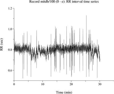	If you have installed plt, you can use the rrplot shell script to view an RR interval time series (obtained using ann2rr). The figure at left was made using the command: rrplot -r mitdb/100 -a atr
	It is often useful to create a histogram of RR intervals, as shown at left. Look in the script rrhist to see how this can be done, using ann2rr together with sort and uniq (both of these utilities are standard components of Unix, GNU/Linux, Mac OS/X, and MS-Windows/Cygwin). The figure at left was made using the command: rrhist -r mitdb/100 -a atr

Discontinuities in an NN interval sequence

There are many reasons why an NN interval sequence may be discontinuous, including poor signal quality, loss of signal, or interruption by ectopic (abnormal) beats. In some cases, careful selection of continuous sequences is sufficient, but even non-cardiogenic interruptions, such as noise, may be correlated with physical activity or symptoms that are in turn correlated with heart rate. For this reason, it is necessary to take care that selection bias is not introduced when discarding noisy data.

To avoid having to discard noisy data, some investigators prefer to reconstruct the missing sinus beat intervals. You can use nguess to do this; as its name implies, nguess makes (reasonable) guesses about the locations of missing beats. At left is an NN time series based on nguess's guesses for the same data shown in the previous plots.

Not all methods for time series analysis require continuous series; some investigators avoid those methods that have such a requirement because they force a choice among poor alternatives. We will return to this subject in the next section.

Extracting Instantaneous Heart Rate from an Annotation File

In clinical practice, heart rate is measured in beats per minute (bpm) and is almost always computed by extrapolation (for example, by counting the beats in a six-second interval and multiplying by ten).

In studies of heart rate variability (HRV), however, heart rate is modelled as as a quasi-continuous signal, and the RR interval series is used to obtain samples of that signal at more frequent intervals.

The simplest and in many ways the best way to do this is to calculate the reciprocal of each interval in minutes; to do so, use ihr. For example, use a command such as

ihr -r ecg01 -a qrs

ihr -r ecg01 -a qrs >ecg01.ihr.txt

If you have installed plt, you can use hrplot to view a heart rate time series (generated on-the-fly by ihr). The figure at left was made using the command: hrplot -r mitdb/100 -a atr See the manual page for hrplot for further details and options.

Most (but not all) methods for frequency-domain analysis of time series require that the series be sampled at uniform intervals. The heart rate time series obtained by ihr is sampled at non-uniform intervals in general (in fact, it is precisely the non-uniformity that one wishes to study). If you plan to study heart rate in the frequency domain, you might want to resample the heart rate signal at uniform intervals. The standard algorithm for doing so, IPFM, is implemented by tach. Use tach to obtain a uniformly sampled heart rate time series with a command such as

tach -r ecg01 -a qrs -F 4

Both ihr and tach offer powerful techniques for outlier rejection, which is almost always needed when studying long heart rate time series. Read their manual pages for details (follow the links above). A problem unique to tach, however, is that once outliers have been rejected, the heart rate samples calculated for those intervals are incorrect and may unduly influence subsequent analysis. For this reason, you may prefer to reconstruct the NN interval time series using nguess (see the previous section) before using tach, or to postprocess tach's output to remove impulse noise, if it is necessary to use tach on noisy data or on data that include ectopic beats.

It should be understood that reconstruction and resampling is a controversial operation for many reasons, and that it is not necessary unless you wish to use certain specific frequency-domain techniques. For example, power spectral density estimation using FFT or maximum entropy (autoregressive) methods requires resampling, but the Lomb-Scargle algorithm does not require resampling, and has other advantages. For further discussion, see this paper.

There is a third approach to study of heart rate time series, which is to use classical frequency-domain algorithms such as the FFT with the irregularly-sampled heart rate time series. This approach, since it treats the time series as a "beat number" series, yields spectra that are not in the frequency domain, but in the sequency (sometimes called "beatquency") domain.

Heart Rate Variability

The commonly quoted scalar measures (SDNN: the standard deviation of NN intervals, pNN50: the fraction of NN intervals that differ by more than 50 ms from the previous NN interval, RMSSD: the root-mean-square of successive differences of NN intervals) offer only a limited view of HRV. PhysioToolkit does not currently offer software for computing these measures, but you can easily compute them from the NN intervals obtained using ann2rr. These measures were developed at a time when the standard technology for assessing HRV was a pair of calipers and a hand calculator. They represent only the aspect of HRV that is visible by inspection of a chart recording. Nevertheless, it is clear from many studies that these simple measures capture significant information that relates to age, health, mental and physical workload, and severity of disease.

The pNNx software package goes beyond the classical time-domain measures, and calculates a family of statistics of which pNN50 is a member. The study that introduced pNNx demonstrated that these statistics can be better discriminators than pNN50 between young and old, periods of wakefulness and sleep, and health and disease.

What these scalar measures do not capture is any information relating to the order of the intervals, except for pairwise coupling. Such information can be obtained only by the use of more sophisticated analyses. Frequency-domain analysis of HRV reveals much more. You may wish to explore HR power spectra obtained using lomb (Lomb-Scargle periodogram estimation), fft (Fourier transform), or memse (maximum entropy/all poles/autoregressive estimation).

	The three spectra above and at left were created using these three methods from the HR time series shown in the previous section. If you have installed plt, you can duplicate these spectra by hrlomb -r mitdb/100 -a atr hrfft -r mitdb/100 -a atr hrmem -r mitdb/100 -a atr See the manual page for hrfft for further details and options.

These samples illustrate the similarities and differences of these techniques. The AR method (memse / hrmem) yields much cleaner spectra than the others; this property is an artifact of the method, however, which models the spectrum using a relatively low-degree polynomial that cannot reproduce fine detail, whether that detail represents the signal or the noise. Although many papers on the subject of HRV contain attractively drawn AR spectra, it is simply not possible to know from a single AR spectrum if the model order was adequate to capture the important frequency components of the input. If you choose to use AR spectra anyway, always check your results against those obtained using one of the other methods illustrated here.

The Lomb and Fourier spectra more closely resemble each other. A unique property of the Lomb method is that it permits estimation of frequency components at higher frequencies than the other methods, because there is no clearly defined Nyquist frequency in a non-uniform time series. The resampling required by the other methods, by contrast, has the side effect of low-pass filtering the time series, so that components above roughly 0.4 Hz are severely attenuated.

Even the best spectral density estimation algorithm cannot save you if the data are contaminated, however. All three of these spectra exhibit this problem. The peaks at 0.167 and 0.28 Hz in this recording have previously been identified as artifacts of the mechanical components of the analog tape recorder and playback unit used for the original recording, and the 0.42 Hz peak in the Lomb spectrum was identified as another recorder drive train frequency, not previously observed as an artifact in a recording.

The important point is that one needs to look at spectra critically. In this case, it's relatively easy to spot these peaks in the Lomb and FFT spectra as impossibly narrow for anything of physiologic origin; in the AR spectrum, however, they can easily be mistaken for peaks that have significance in terms of physiology, such as the broad peak centered around 0.33 Hz that reflects respiratory sinus arrhythmia (RSA). This peak is visible in the Lomb spectrum at upper left, obtained from the same data as above, in which the power spectrum has been log-transformed; note that this peak is not readily apparent in the log-transformed FFT and MEM spectra above and at left.

The frontiers of research in HRV measurement lie in applications of techniques such as approximate entropy (ApEn), sample entropy (SampEn), detrended fluctuation analysis (DFA), information-based similarity (IBS), multiscale entropy (MSE) analysis, and multifractal analysis. These methods may be capable of revealing features of HRV that are not exposed using other methods of analysis, and that may have diagnostic and predictive value complementary to that obtainable using other methods.

There is no general agreement about how to characterize (or how to interpret) heart rate variability. By choosing to study HRV, you will need to make choices about the algorithms that you use, how to prepare the input to those algorithms, and what to do with their output.